Your stomach rumbles. Do you go to the Italian restaurant that you know and love, or the new Thai place that just opened up? Do you take your best friend, or reach out to a new acquaintance you’d like to get to know better? This is too hard—maybe you’ll just stay home. Do you cook a recipe that you know is going to work, or search the Internet for new inspiration? Never mind, how about you just order a pizza? Do you get your “usual,” or ask about the specials? You’re already exhausted before you get to the first bite. And the thought of putting on a record, watching a movie, or reading a book —which one?—no longer seems quite so relaxing. Every day we are constantly forced to make decisions between options that differ in a very specific dimension: do we try new things or stick with our favorite ones?

This is famously known as the exploration vs. exploitation dilemma. Not just in real life, it also exists in machine learning. This is where the idea of Upper Confidence Bound stands. It can help to solve(to a great extent) this dilemma.

In this tutorial, I will explain to you the application of the Upper Confidence Bound(UCB) algorithm to solve the Multi Bandit problem and show you the whole coding process in Python. Let's dive into the tutorial!

Exploration Vs. Exploitation: The Multi-Armed Bandit Problem

What is Multi-Armed Bandit and How It Works?

This is a use case of reinforcement learning, where we are given a slot machine called a multi-armed bandit. The slot machines in casinos are called bandit as it turns out all casinos configure these machines in such a way that all gamblers end up losing money! Here each arm has its own rigged probability distribution of success. Pulling any one of these arms gives you a stochastic reward of either 1, for success or 0, for failure. Now your task is to find such an optimal strategy that will give you the highest rewards in the long run without the prior knowledge of the probability distribution of success of the machines.

This problem can be related to more business examples such as displaying the optimal ads to the viewer.

So in this tutorial, we are going to solve a use case of the multi-armed bandit problem. We take an example of an online advertising campaign dataset where we have 10 different versions of a similar ad. You see the dataset looks similar to that of a multi-armed bandit problem!

Let's have a quick check on our version of the multi-armed bandit problem-

You can download the dataset from here.

Upper Confidence Bound Intuition

You can find the best option by using an A/B test. Where you can show a different ad to a user and take his feedback, that is whether the user clicks or not. And summing up all the feedback, you can find the best ad to display. Bat wait! There is a problem. In A/B test you are incurring more cost and time by doing exploration and exploitation separately. So we need to combine exploration and exploitation and get the result as soon as possible. We do not have enough time and money to actually do this exploitation, so we will do this during the campaign.

The Upper Confidence Bound algorithm is the kind of algorithm that helps us to perform exploitation and exploration together.

How the UCB Algorithm Works?

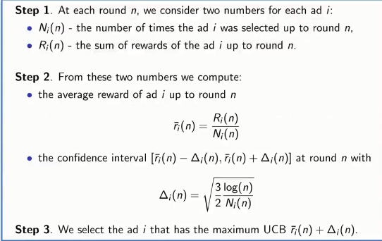
At the start of the campaign, we don't know what is the best arm or ad. So we cannot distinguish or discriminate any arm or ad. So the UCB algorithm assumes they all have the same observed average value. Then the algorithm creates a confidence bound for each arm or ad. So it randomly picks any of the arms or ads. Then two things can happen- the user clicks the ad or the arm gives a reward or does not. Let's say the ad did not have a click or the arm was a failure. So the observed average of the ad or arm will go down. And the confidence bound will also go down. If it had a click, the observed average would go up and the confidence bound also goes up. By exploiting the best one we are decreasing the confidence bound. As we are adding more and more samples, the probability of other arms or ad doing well is also going up. This is the fundamental concept of Upper Confidence Bound algorithm.

Now let's see what steps are involved to perform this algorithm on our dataset:

Implementing the Multi-Armed Bandit Problem in Python

We will implement the whole algorithm in Python. First of all, we need to import some essential libraries.

# Importing the Essential Libraries 
import numpy as np
import matplotlib.pyplot as plt
import pandas as pd

Now, let's import the dataset-

# Importing the Dataset 
dataset = pd.read_csv('Ads_CTR_Optimisation.csv')

Now, implement the UCB algorithm:

# Implementing UCB
import math
N = 10000
d = 10
ads_selected = []
numbers_of_selections = [0] * d
sums_of_rewards = [0] * d
total_reward = 0
for n in range(0, N):
    ad = 0
    max_upper_bound = 0
    for i in range(0, d):
        if (numbers_of_selections[i] > 0):
            average_reward = sums_of_rewards[i] / numbers_of_selections[i]
            delta_i = math.sqrt(3/2 * math.log(n + 1) / numbers_of_selections[i])
            upper_bound = average_reward + delta_i
        else:
            upper_bound = 1e400
        if upper_bound > max_upper_bound:
            max_upper_bound = upper_bound
            ad = i
    ads_selected.append(ad)
    numbers_of_selections[ad] = numbers_of_selections[ad] + 1
    reward = dataset.values[n, ad]
    sums_of_rewards[ad] = sums_of_rewards[ad] + reward
    total_reward = total_reward + reward

# ads_selected = [], is used to append the different types of ads selected in each round 
# numbers_of_selections = [0] * d, is used to count the number of time an ad was selected 
# sums_of_rewards = [0] * d, is used to calculate the cumulative sum of rewards at each round

As we don't have any prior knowledge about the selection of each ad, we will take the first 10 rounds as trial rounds. So, we set the if condition:  if (numbers_of_selections[i] > 0) so that the ads are selected at least once before entering into the main algorithm.

Then we implement the second step of the algorithm, computing the average reward of each ad I up to round n and the upper confidence bound for each ad.

Here we applied a trick in the else condition by taking the variable upper_bound  to a huge number. This is because we want the first 10 rounds as trial rounds where the 10 ads are selected at least once. This trick will help us to do so.

After 10 trial rounds, the algorithm will work as the steps explained earlier.

Visualizing the Result

plt.hist(ads_selected)
plt.title('Histogram of ads selections')
plt.xlabel('Ads')
plt.ylabel('Number of times each ad was selected')
plt.show()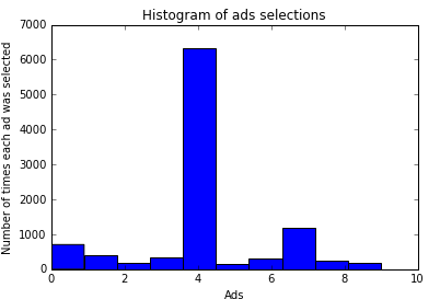

From the above visualization, we can see that the fifth ad got the highest click. So our model advice us to place the fourth version of the ad to the user for getting the highest number of clicks!

Multi-Armed Bandit VS. A/B Testing: Which to choose?

A/B testing sounds simple. Suppose you are running the above ad campaign for an A/B test. Here, you split the samples in half. Provide 50% of the customer with one version of the ad and the other 50% with another. Run it for a specific period of time. After that period calculate the impressions on each ad. The highest one is the winner.

But here is a problem. You are completely isolating the exploration to exploitation. You are wasting resources and losing variation while trying to find the winner with this approach.

Here Bandit algorithms can help. It is sometimes called learning while earning means you are making money when you are also making progress to find the winner. In a shorter period of time, it provides you amazing performance. Take an example. You are running an ad campaign for Black Friday sales. You have only a week and still don't know which ad will get the best performance. Here you should not perform A/B testing. Why? Because you have limited time and not enough data to perform the test. Instead, follow a multi-armed bandit approach. It performs extremely well for shorter periods of time.

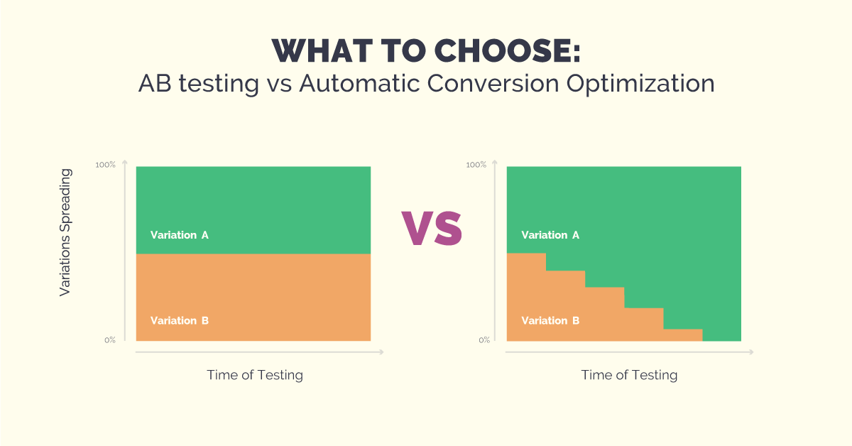
Surprisingly, it performs great in longer periods too! Unlike the A/B testing approach, it gradually searches for the best one. This makes the process faster and smoother. And nonetheless, does not make the customers annoyed like in A/B testing where 50% of the customers are provided with inferior variations.

The only disadvantage with a bandit algorithm is that it is computationally complex. But yet it gives you the perfect sense of customization while you are dealing with a lot of optimizing tasks.

There are successful companies that are implementing the bandit concepts to making money! Take Optimizely for instance, they provide multi-armed bandit solutions for ad campaign optimization. How successful they are?

Well, In 2012 presidential election cycle, they worked for both the Obama re-election campaign and the campaign of Republican challenger Mitt Romney!

Applications of Multi-Armed Bandit in Real Life

Whenever you stuck in a situation where you need to choose an optimal decision among all the existing options, that is a multi-armed bandit problem. You should stick to the sub-optimal option and yet you need to seek the best one. This problem is countered in many aspects of real life such as health, finance, pricing, and so on. The followings are some of the real-life examples where we can use the bandit strategy-

Healthcare In the time of the clinical trial of treatments, collecting data for assessing the effect on animal models during the full range of disease stages can be difficult.  Since poor treatments can cause deterioration of the subject’s health. This problem can be seen as a contextual bandit problem. Here an adaptive allocation strategy is used to improve the efficiency of data collection by allocating more samples for exploring promising treatments. This is a practical application of the multi-armed bandit algorithm.

Finance In recent years, sequential portfolio selection has been an important issue in the field of quantitative finance. Here, the goal of maximizing cumulative reward often poses the trade-off between exploration and exploitation. In this research paper, the authors proposed a bandit algorithm for making online portfolio choices by exploiting correlations among multiple arms. By constructing orthogonal portfolios from multiple assets and integrating their approach with the upper-confidence-bound bandit framework, the authors derive the optimal portfolio strategy representing a combination of passive and active investments according to a risk-adjusted reward function.

Dynamic Pricing Online retailer companies are often faced with the dynamic pricing problem: the company must decide on real-time prices for each of its multiple products. The company can run price experiments (make frequent price changes) to learn about demand and maximize long-run profits. The authors in this paper propose a dynamic price experimentation policy, where the company has only incomplete demand information. For this general setting, authors derive a pricing algorithm that balances earning an immediate profit vs. learning for future profits. The approach combines a multi-armed bandit with partial identification of consumer demand from economic theory.

Anomaly Detection Performing anomaly detection on attributed networks concerns with finding nodes whose behaviors deviate significantly from the majority of nodes. Here, the authors investigate the problem of anomaly detection in an interactive setting by allowing the system to proactively communicate with the human expert in making a limited number of queries about ground truth anomalies. Their objective is to maximize the true anomalies presented to the human expert after a given budget is used up. Along with this line, they formulate the problem through the principled multiarmed bandit framework and develop a novel collaborative contextual bandit algorithm, that explicitly models the nodal attributes and node dependencies seamlessly in a joint framework, and handles the exploration vs. exploitation dilemma when querying anomalies of different types. Credit card transactions predicted to be fraudulent by automated detection systems are typically handed over to human experts for verification. To limit costs, it is standard practice to select only the most suspicious transactions for investigation.

Algorithm Selection Algorithm selection is typically based on models of algorithm performance, learned during a separate offline training sequence, which can be prohibitively expensive. In recent work, they adopted an online approach, in which a performance model is iteratively updated and used to guide selection on a sequence of problem instances. The resulting exploration-exploitation trade-off was represented as a bandit problem with expert advice, using an existing solver for this game, but this required using an arbitrary bound on algorithm runtimes, thus invalidating the optimal regret of the solver. In this research, a simpler framework was proposed for representing algorithm selection as a bandit problem, using partial information and an unknown bound on losses. 

Final Thoughts

In this multi-armed bandit tutorial, we discussed the exploration vs. exploitation dilemma. We popularized the approach to solve this problem with the Upper Confidence Bound algorithm. Then we implemented this algorithm in Python. We considered the differences between a multi-armed bandit and A/B testing and found out which one is the best for both long-term and short-term applications. Finally, we see the applications of multiple-armed bandit in various aspects of our real life.

Hope this article helped you to grab the concepts of this phenomenon. Please share your thoughts on this discussion in the comments.

Happy Machine Learning!