A Beginners Guide to Logistic Regression(with Example Python Code) | Machine Learning

In this article, we will go through the concept of logistic regression, a simple classification algorithm. Then we will implement the algorithm in Python.

Logistic Regression Intuition:

Logistic Regression is the appropriate regression analysis to solve binary classification problems( problems with two class values yes/no or 0/1). This algorithm analyzes the relationship between a dependent and independent variable and estimates the probability of an event to occur. Like other regression models, it is also a predictive model. But there is a slight difference. While other regression models provide continuous output, Logistic Regression is used to model the probability of a certain class or event existing such as pass/fail, win/lose, alive/dead or healthy/sick.

A good example can be finding the probability of getting cancer(yes/no) by a person for smoking for some years based on the dataset of people containing their smoking period, age, and the condition(having cancer or not).

How this Algorithm Works?

If you remember the regression, you can understand that in regression, we use a function to predict the probability of an event to occur. In logistic regression, the idea is the same but with that function, we combine another function named sigmoid or logistic function to find the probability. You can better understand from the following illustration-

                                          

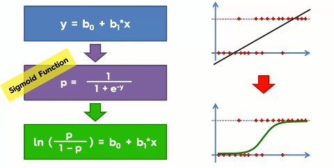
Top of the illustration you can see the original regression equation(at left) and the resulting regression line(at the right of the top). And when we combine it with the sigmoid function we get the logistic equation(in the green box at the bottom). And the resulting slope is shown at the bottom right.

Well, with this logistic function you will get the probability of an event to occur like the probability of buying a car by a person of a certain age.

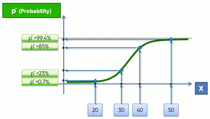
Here, you can see that people of a lower age(between 20 to 30) are less likely to buy a car(between 0.7% to 23%) whereas people of higher ages have more probability.

But wait! We are doing classification and we want the probability of people buying a car or not(yes/no values) but here we get a continuous probability. So what would we do is that we will take a threshold point(like 50% or 0.5) in the graph and based on that line we will calculate the probability.

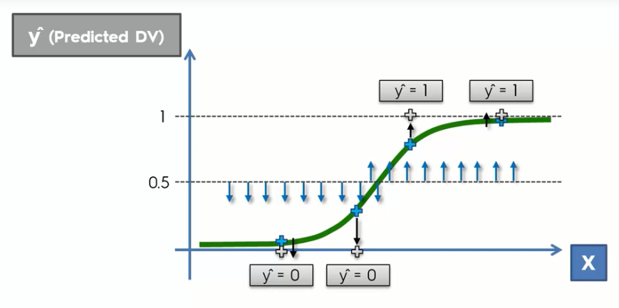
Here you can see we take a threshold point(50% or 0.5) where anything under that probability classified as a 0 or no value and above that line the probability is classified as 1 or yes.

This way we can use a regression function to solve classification problems.

Logistic Regression in Python :
Now we will implement this algorithm in Python. Here we take a dataset containing the Age, Salary, and Action(yes/no value) of purchasing a car. Now our task is to classify a person in terms of his Age and Salary whether he/she is supposed to buy the car.

You can download the dataset from here.

First of all, we import essential libraries. You will get the code in Google Colab also.

# Importing Essential Libraries 
import numpy as np
import matplotlib.pyplot as plt
import pandas as pd

Now, we will import the dataset to our program.

# Importing the Dataset 
dataset = pd.read_csv('Social_Network_Ads.csv')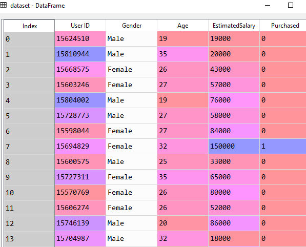

                                                           

In this dataset, the Age and EstimatedSalary column are independent variables and the last column Purchased is the dependent variable. The last column contains the values 0 or 1. It means it provides the output like yes or no.

Now we take the indexes of Age and EstimatedSalary as our independent variable matrix. And take the Purchased column in the dependent variable vector.

X = dataset.iloc[:, [2, 3]].values
y = dataset.iloc[:, 4].values

Now we split the dataset into a training set and a test set. For this, we take the test size=0.25%. And execute it. After execution, we get 300 training sets and 100 test sets.

# Splitting the Dataset into Training and Test Set 
from sklearn.model_selection import train_test_split
X_train, X_test, y_train, y_test = train_test_split(X, y, test_size = 0.25, random_state = 0)

Now, we will do feature scaling. To transform the x_train matrix object to scale, we use the fit_transform method.

# Scaling the Datasets
from sklearn.preprocessing import StandardScaler
sc = StandardScaler()
X_train = sc.fit_transform(X_train)
X_test = sc.transform(X_test)

 Now, we fit a logistic regression to the training set. We use the linear model library to import the class LogisticRegression. Then we create the classifier object and call that object.

# Fitting the Datataset with Regression Class 
from sklearn.linear_model import LogisticRegression
classifier = LogisticRegression(random_state = 0)
classifier.fit(X_train, y_train)

Note: Here we set the random_state to zero so that the result in our program and yours remain the same.

Well, we have come to the final part of the algorithm. Let's create a variable to predict the result.

# Predicting the output 
y_pred = classifier.predict(X_test)

Now, we will see how good our model is to predict the values. Let's evaluate our model using the confusion matrix.

# Building the Confusion Matrix 
from sklearn.metrics import confusion_matrix
cm = confusion_matrix(y_test, y_pred)

                                                         

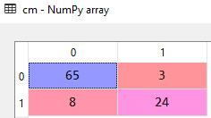
Here the output shows us that the model predicted 89 (65 + 24) correct and 11(8 + 3) incorrect values. So the accuracy of the model is 89%, pretty impressive!

Now we will visualize the result of our model.

# Visualising the Test set results
from matplotlib.colors import ListedColormap
X_set, y_set = X_test, y_test
X1, X2 = np.meshgrid(np.arange(start = X_set[:, 0].min() - 1, stop = X_set[:, 0].max() + 1, step = 0.01),
                     np.arange(start = X_set[:, 1].min() - 1, stop = X_set[:, 1].max() + 1, step = 0.01))
plt.contourf(X1, X2, classifier.predict(np.array([X1.ravel(), X2.ravel()]).T).reshape(X1.shape),
             alpha = 0.75, cmap = ListedColormap(('red', 'green')))
plt.xlim(X1.min(), X1.max())
plt.ylim(X2.min(), X2.max())
for i, j in enumerate(np.unique(y_set)):
    plt.scatter(X_set[y_set == j, 0], X_set[y_set == j, 1],
                c = ListedColormap(('red', 'green'))(i), label = j)
plt.title('Logistic Regression (Test set)')
plt.xlabel('Age')
plt.ylabel('Estimated Salary')
plt.legend()
plt.show()

                                                      

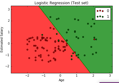
Here the graph shows us the classification of purchasing a car or not based on various Ages and EstimatedSalary.