Convolution Neural Network | Machine Learning

Convolution Neural Network: A Convolutional neural network (CNN, or ConvNet) is a class of deep, feed-forward artificial neural networks, most commonly applied to analyzing visual imagery.

CNN's use a variation of multilayer perceptrons designed to require minimal preprocessing. They are also known as shift invariant or space invariant artificial neural networks (SIANN), based on their shared-weights architecture and translation invariance characteristics.

Convolutional networks were inspired by biological processes in that the connectivity pattern between neurons resembles the organization of the animal visual cortex. Individual cortical neurons respond to stimuli only in a restricted region of the visual field known as the receptive field. The receptive fields of different neurons partially overlap such that they cover the entire visual field.

CNN uses relatively little pre-processing compared to other image classification algorithms. This means that the network learns the filters that in traditional algorithms were hand-engineered. This independence from prior knowledge and human effort in feature design is a major advantage.

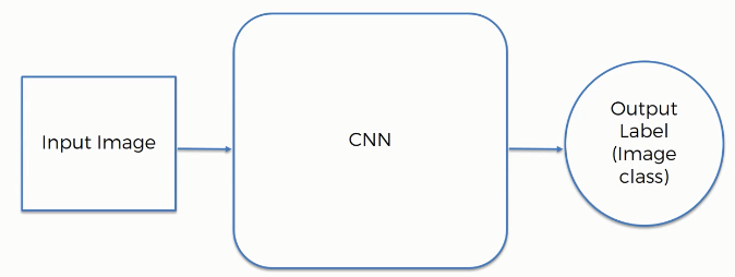
Here, we have an image, convolution neural network and having output label image.

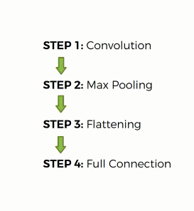
Convolution Operation: In this tutorial, we are going to talk about convolution. Here, we describe the convolution function:

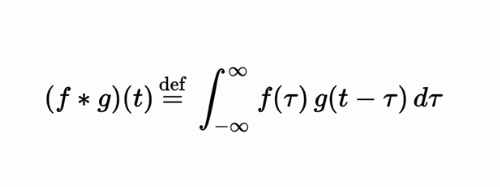
Convolution is a combined integration of the two functions and it shows you how one function modifies the other or modifies the shape of the other.

Convolution is a mathematical operation to merge two sets of information. In our case, the convolution is applied to the input data using a convolution filter to produce a feature map. There are a lot of terms being used so let's visualize them one by one.

On the left side is the input to the convolution layer, for example, the input image. On the right is the convolution filter, also called the kernel, we will use these terms interchangeably. This is called a 3x3 convolution due to the shape of the filter.

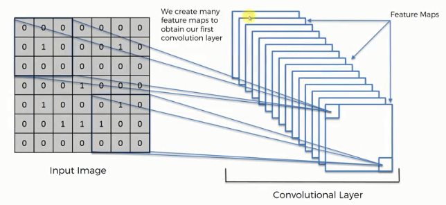
We perform the convolution operation by sliding this filter over the input. At every location, we do element-wise matrix multiplication and sum the result. This sum goes into the feature map. Now, we have some input messages and we create a feature map. We create multiple feature maps because we use different filters.

ReLU  Layer: In this tutorial, we are going to talk about the ReLU layer. Here, we are applying the rectifier because we want to increase non-linearity in our image. They propose different types of rectified functions.

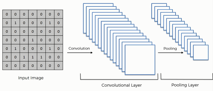
Pooling: In this tutorial, we are going to talk about the max pooling.

Max pooling is a sample-based discretization process. The objective is to down-sample an input representation (image, hidden-layer output matrix, etc.), reducing its dimensionality and allowing for assumptions to be made about features contained in the sub-regions binned.

This is done so in part to help over-fitting by providing an abstracted form of the representation. As well, it reduces the computational cost by reducing the number of parameters to learn and provides basic translation invariance to the internal representation.

Max pooling is done by applying a max filter to (usually) non-overlapping subregions of the initial representation.

We are taking the maximum of the pixel that we or the values that we have. This helping with preventing overfitting. We applied the convolution operation and now we apply the pooling.

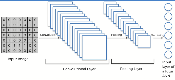
Flattening: Here, we have the pooled featured map. After that, we apply the convolution operation to our image and then we apply the pooling to the result of the collision. So, we are going to flatten it into the column. Here, we see many pooling layers. We put them into one log column sequentially. In the input image, we apply the convolution. And also apply the rectifier function.

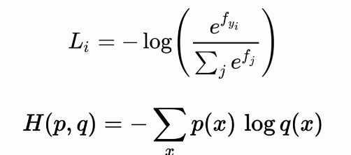
Full Connection: Today, we are talking about the full connection. In this step, we are adding a whole artificial neural network to our convolutional neural network. Here, we are calling them fully connected which are the hidden layer. The main purpose of the artificial neural network to combine our features into more attributes. Here, we used to call a cost function in an artificial neural network and we used mean square error there is a common illusional neural network. It is called a loss function and we use the across entropy function for that. We are trying to optimize it to minimize that function to optimize our network. We had an artificial neural network that is backpropagated and some things are adjusted t help optimize. It all done through gradient descent of backpropagation. The dog neuron knows that the answer is actually a dog because at the end we are comparing to the picture or to the label on the picture.

CNN in Python 1: In this tutorial, we are going to implement CNN in python. Here, we build our convolutional neural network model, we will simply need to change the image of

Then, we will be able to train a convolutional neural network to predict if some new brain image contains the tumor is yes or no. Now, we have to input these images in our convolution neural that work.

Here, in the working directory, we have a dataset that is all our images of cats and dogs. In each folder the training set and the test set we would get for example 5000 images.

The first pillar of the structure is to separate our images into two separate folders. A training set folder and testing set folder. Here, we see different dog pictures. Now, we can take some pictures of our friends and replace these dogs' pictures with that picture. Then, we will able to train an algorithm that will predict. And, there are images of a cat. Here, the training set contained 8000 customers and the test set contained 2000 customers. Here, also,4000 images for dogs and 4000 images for cats. So, there are an 80 percent and 20 percent split. We already import this dataset. we do not need to encode the dataset because the independent variable is some way of a pixel and the three-channel. We need to split the dataset into the training set and test set. Now, we need to apply the feature scaling. You will get the code in Google Colab also.

# Importing the libraries
import tensorflow as tf
from keras.preprocessing.image import ImageDataGenerator

# Downloading the dataset

You can download the dataset zip from here with 5000 pictures and train and test datasets. Download the zip file and extract it in your project directory. 

CNN in Python 2: In this tutorial, we are going to talk about the convolution neural network. The first step is to import all the Keras packages that we will need to make our CNN model. Here, the first package is sequential. We use sequential packages to initialize our neural network. Now, we import convolution layers and we are working on images and since images are in two dimensions. We use the 2D packages to deal with images. And we also add our pooling layers. And next is flatten. Here, we also use the last dense packages. We use to add fully connected layers and a classic artificial neural network. Now, I execute the code.

Now, we are going to create an object of this sequential class. We are going to call this object classifier and we call the sequential method.

from keras.models import Sequential
from keras.layers import Convolution2D
from keras.layers import MaxPooling2D
from keras.layers import Flatten
from keras.layers import Dense

CNN in Python 3: Now, we are going to preprocess our data. Here we will preprocess our train set and test set.

# Preprocessing the Training set
train_datagen = ImageDataGenerator(rescale = 1./255,
                                   shear_range = 0.2,
                                   zoom_range = 0.2,
                                   horizontal_flip = True)
training_set = train_datagen.flow_from_directory('dataset/training_set',
                                                 target_size = (64, 64),
                                                 batch_size = 32,
                                                 class_mode = 'binary')

# Preprocessing the Test set
test_datagen = ImageDataGenerator(rescale = 1./255)
test_set = test_datagen.flow_from_directory('dataset/test_set',
                                            target_size = (64, 64),
                                            batch_size = 32,
                                            class_mode = 'binary')

 

CNN in Python 4: In this tutorial, we are going to take care of the first state of convolutions. Here, we take the classifier object and also include the method add. Here, we include convolution2D. Here, we use the 32 feature detectors three by three-dimension for feature detectors. We need to specify what are the expected format of our input images. The input image converted into a 3D array if the image is a color image and into a 2D array if it is a black and white image. The 3D means three-channel. We need to start with the 2D array dimension. We need to import here for our input shape argument. Therefore, 64 to 64 and then the number of channel 3 that is we are using tensor flow. We have one last argument to input which is the activation function exactly as we did for our fully connected layers. We used this activation function to activate the neurons in the neural network. Here, we are using the rectifier function.

# Initialising the CNN

cnn = tf.keras.models.Sequential()

# Step 1 - Convolution

cnn.add(tf.keras.layers.Conv2D(filters=32, kernel_size=3, activation='relu', input_shape=[64, 64, 3]))

CNN in Python 5: Today, we will take care of the second step pulling. We call the classifier. For the classifier object, we use the add method. And we add the new parenthesis max pooling. We use the max pool size 2 and 2.This line will reduce the size of our maps and it's well divided by two. The size of the feature map is divided by two. For flattening, we use the classifier object and use the add method. We use the parenthesis Flatten().

In the same way, For Full connection, we use the classifier object and use the add method. We use the parenthesis Dense (). Also has a parenthesis output_dim is equal to 128. We need to choose a number that is not too small to make the classifier a good model and also not too big. Here, we will go with these 128 hidden nodes in the hidden layer. And another activation function is a rectifier. Now, we copy-paste the code. And, add the sigmoid function. now, we add 128 to 1. Then, we get the final layer, which predicts the output.

# Step 2 - Pooling

cnn.add(tf.keras.layers.MaxPool2D(pool_size=2, strides=2))

# Adding a second convolutional layer

cnn.add(tf.keras.layers.Conv2D(filters=32, kernel_size=3, activation='relu'))
cnn.add(tf.keras.layers.MaxPool2D(pool_size=2, strides=2))

# Step 3 - Flattening

cnn.add(tf.keras.layers.Flatten())

# Step 4 - Full connection

cnn.add(tf.keras.layers.Dense(units=128, activation='relu'))

# Step 5 - Output Layer

cnn.add(tf.keras.layers.Dense(units=1, activation='sigmoid'))

CNN in Python 8: In this tutorial, we need to compile the whole thing by choosing to cast a grade. To compile this, we add the compile method and also add the parameter in the optimizer. The optimizer is equal to Adam. Ans we use loss is equal to bunary_cross entropy. And, the metrics are equal to the accuracy.

# Compiling the CNN

cnn.compile(optimizer = 'adam', loss = 'binary_crossentropy', metrics = ['accuracy'])

# Training the CNN on the Training set and evaluating it on the Test set

cnn.fit(x = training_set, validation_data = test_set, epochs = 25)

CNN in Python 9: In this tutorial, we are going to fit the CNN image. We actually need a lot of images to find and generalize some correlations. The amount of our training images is augmented because the transformation is a random transformation. Image augmentation is a technique that allows you to enrich our dataset our train set. Now, image augmentation is applied to the training set. Here, we create ImageDataGenerator class. We will rescale all our pixel values between 0 and 1. By rescaling them using this rescale equals one over 255 then all our pixels will be between 0 and 1. She arranged that to apply random transaction and we will keep this open to value zoom range. So these 0.2 values here are just some parameters of how much we want to apply these random transformations. We call it the test set because this code section will create the test set. We have 8000 images in our training set. we need to replace 2000 with 8000 right. Now, we generate a fit method for our classifier. Now, we execute it. And we create another object. Here, 8000 and 2000 images belonging to two classes.2000 image of our test set. After execution, we get 75% accuracy. We get three predictions out of four..there is a difference between the accuracy in the training set and accuracy in the test set.

import numpy as np
from keras.preprocessing import image
test_image = image.load_img('dataset/single_prediction/cat_or_dog_1.jpg', target_size = (64, 64))
test_image = image.img_to_array(test_image)
test_image = np.expand_dims(test_image, axis = 0)
result = cnn.predict(test_image)
training_set.class_indices
if result[0][0] == 1:
    prediction = 'dog'
else:
    prediction = 'cat'
print(prediction)

CNN in Python 10: In this tutorial, we are going to talk about if we achieve our goal to get an accuracy of more than 80 percent on the test. Only adding a convolutional layer, we will see how it will definitely improve our performance results. Now, we add another convolution layer. Here, we going to keep the same parameter. Now, we execute the whole code. The accuracy of the training set is about 85. The accuracy of stains on the test began at 55 percent almost 56 percent. We got indeed 64 percent and 68 percent on the test set. We get an accuracy of 85 percent for the training set and 82 percent for the test. We get a difference of 3 percent as opposed to this 10 percent difference that we got in.

Softmax and Cross-Entropy: In softmax function in order to help us out of the situation.

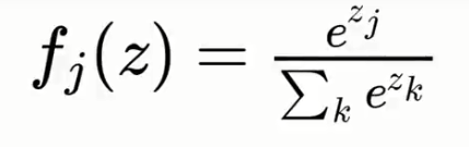
The softmax function or the normalized exponential function is a generalization of the logistic function. It takes the exponent and puts the power of zed and adds it up so that one's two across all. Here we use a function called the mean squared which we used as the cost function for assessing our natural performance. Our goal is to minimize the MSE in order to optimize our network performance.