K-Nearest Neighbor in 4 Steps(Code with Python & R) | Machine Learning

There is a proverb-

"Birds of a feather flock together"

It means same things remain in a common group. I don't know where this proverb has its origin. But the algorithm we are going to get introduced has some sort of similarity with this proverb. It is K nearest neighbor aka KNN. KNN is a simple and widely used machine learning algorithm based on similarity measures of data. That is it assumes a data point to be a member of a specific class to which it is most close. 

In this tutorial, we will learn about the K-Nearest Neighbor(KNN) algorithm. Then we will implement this algorithm in Python and R. Let's dive into it!

What is KNN in Machine Learning?

K-nearest neighbor is a non-parametric lazy learning algorithm, used for both classification and regression. KNN stores all available cases and classifies new cases based on a similarity measure. The KNN algorithm assumes that similar things exist in close proximity. In other words, similar things are near to each other. When a new situation occurs, it scans through all past experiences and looks up the k closest experiences. Those experiences (or: data points) are what we call the k nearest neighbors of a data point. It measures the neighbors using some distance functions popularly Euclidian distance. The majority of those neighbors will determine the class of a new instance of data i.e. the instance will represent that category or class of the majority of neighbor data.

How KNN Algorithm Works?

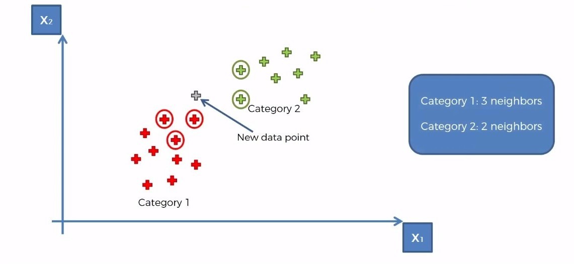
Let's take an example where we have some data points of two different classes. Now our task is to determine the position of a new data point whether it falls in the red category or the green category.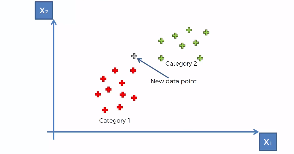

                                                 

Here where KNN algorithm comes into action. There are four steps to perform a complete KNN algorithm. They are-

• Choose the number of K, where k represents the number of neighbors
• Measure the distance of K closest neighbors of the data point
• Counts the number of neighbors of each category
• Assign the new data point to the category of most number of neighbors

Choosing a Distance Metric for KNN Algorithm

There are many types of distance metrics that have been used in machine learning for calculating the distance. Some of the common distance metrics for KNN are-

• Euclidian Distance
• Manhattan Distance
• Minkowski Distance

But Euclidian distance is the most widely used distance metric for KNN. In our tutorial, we will also use this distance metric.

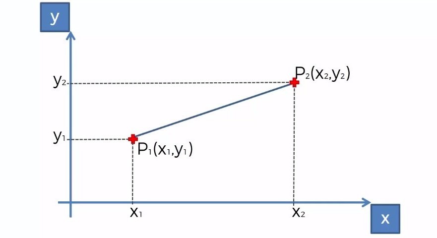
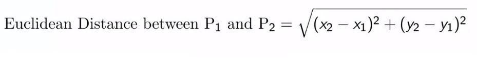
Euclidean distance is a basic type of distance that we define in geometry. The distance between two points is measured according to this formula.

Let's apply the above steps on our data to find the category of the new data point.

Step 1: Choose the number of K neighbors, say K = 5

Step 2: Take the K = 5 nearest neighbors of the new data point according to the Euclidian distance

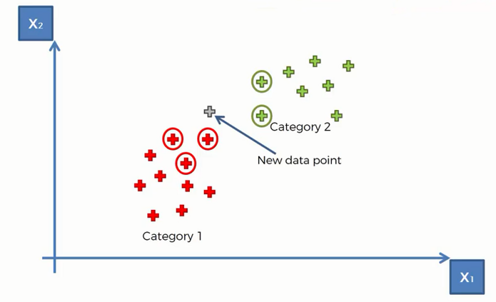
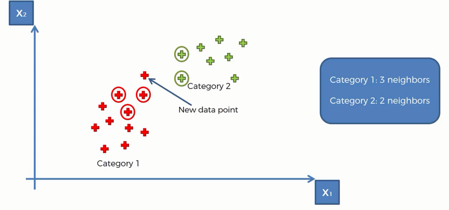
Step 3: Among these K neighbors, count the members of each category

Step 4: Assign the new data point to the category that has the most neighbors of the new data point. Here it is the red category-

Characteristics of KNN Algorithm

First of KNN is a supervised machine learning algorithm and probably one of the simplest algorithms for classification and regression. It has some unique features. Let's take a look at them-

• Lazy Learning Algorithm- KNN is called "Lazy Learning Algorithm" because it does not require a training phase. It does all the calculations in the prediction stage. Rather than learning from the training data, it kinds of 'memorize' them and every time making a prediction search the k nearest neighbors in the entire dataset. That is why it has no specific training time.
• Non-Parametric Algorithm It is a non-parametric algorithm because it does not require parameters. More precisely, it does not assumes anything about the underlying property of data. This is because the KNN based model does not learn anything from the data in the training stage.
• Instance-Based Learning It does not have a specific training stage. It uses all the training instances while making the prediction. That is why often we call it an instance-based or case-based learning algorithm. 

Choosing an Optimal Value of K in KNN

There is no definite way to choose the best value of K. You need to choose a value for K that is larger enough to avoid noise and smaller enough not to include instances of other classes. Though it is hard to choose an optimal value, there are some heuristic methods available to use to find the best value of K for your particular model.

• Square Root Method The most common method is to take the square root value of the total number of training instances of your data set. The rule of thumb is to take an odd number. The method just works fine almost every time.
• Hyperparameter Tuning K is a hyperparameter of the KNN algorithm(a hyperparameter is a property of the model provided by the user). You can apply tuning methods such as a grid search to find the optimal value. For this, taken the same data separately(do not use the test data) and apply fit a KNN model with a grid search to find the value of K that perfectly works for your problem.
• Schwarz Criterion This is the most advanced thing you can do. This criterion works by minimizing the distortion added with a multiplied value of some other factors including the number of clusters, the dimension of the problem, and the total number of data points.

Sometimes you may hear about the "Elbow Method" to find K. This method is used in K-means Clustering, an unsupervised learning algorithm to find the optimal number of clusters, K. But it is not a useful method for KNN.

Implementing KNN in Python

Now we will implement the KNN algorithm in Python. We will use the dataset Social_Network_Ads.csv

You can download the dataset from here.

First of all, we will import all the essential libraries. You will get the code in Google Colab also.

import numpy as np 
import matplotlib.pyplot as plt 
import pandas as pd

Now, let's import our dataset.

dataset = pd.read_csv('Social_Network_Ads.csv')

Let's have a look on our dataset.

                    

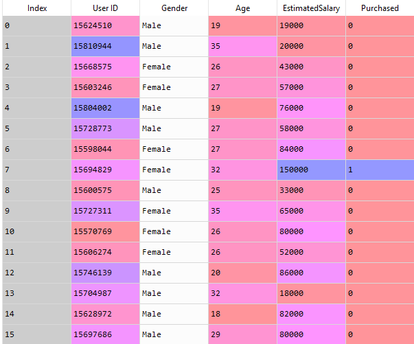
Here you can see that the Age and EstimatedSalary columns are independent variables and the Purchased column is the dependent variable. So we will take the Age and EstimatedSalary in the independent variable matrix and the Purchased column in the dependent variable vector.

X = dataset.iloc[:, [2, 3]].values
y = dataset.iloc[:, 4].values

Now, we will split our dataset into train and test sets.

from sklearn.model_selection import train_test_split
X_train, X_test, y_train, y_test = train_test_split(X, y, test_size = 0.25, random_state = 0)

Note: Here random_state parameter is set to zero so that your result and our result remain the same.

We need to scale our training and test set to make sure that they have a standard difference in them.

from sklearn.preprocessing import StandardScaler 
sc = StandardScaler() 
X_train = sc.fit_transform(X_train) 
X_test = sc.transform(X_test)

It's time to make a classifier using the KNN algorithm. To do so we need the following code.

from sklearn.neighbors import KNeighborsClassifier 
classifier = KNeighborsClassifier(n_neighbors = 5, metric = 'minkowski', p = 2) 
classifier.fit(X_train, y_train)

We have come to the final part of our program, lets take a variable to predict the outcome from our model.

y_pred = classifier.predict(X_test)

Now, we use the confusion metrics to find the correct and incorrect prediction. 

from sklearn.metrics import confusion_matrix
cm = confusion_matrix(y_test, y_pred)

Let's execute the code.

                                                                

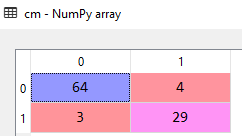
After executing the code, we get 64+29= 93 correct predictions and 3+4=7 incorrect predictions. The correctness of the model is 93% quite impressive!

Well, it's time to look at the result whether it is linear or non-linear.  If it is linear we get a straight line and if it is non-linear we get the curve shape. Let's visualize the outcome.

First, we will visualize our training set.

# Visualising the Training set results 
from matplotlib.colors import ListedColormap 
X_set, y_set = X_train, y_train 
X1, X2 = np.meshgrid(np.arange(start = X_set[:, 0].min() - 1, stop = X_set[:, 0].max() + 1, step = 0.01), 
np.arange(start = X_set[:, 1].min() - 1, stop = X_set[:, 1].max() + 1, step = 0.01)) 
plt.contourf(X1, X2, classifier.predict(np.array([X1.ravel(), X2.ravel()]).T).reshape(X1.shape), alpha = 0.75, 
cmap = ListedColormap(('red', 'green'))) 
plt.xlim(X1.min(), X1.max()) 
plt.ylim(X2.min(), X2.max()) 

for i, j in enumerate(np.unique(y_set)): 
    plt.scatter(X_set[y_set == j, 0], X_set[y_set == j, 1], c = ListedColormap(('red', 'green'))(i), label = j) 

plt.title('K-NN (Training set)') 
plt.xlabel('Age') 
plt.ylabel('Estimated Salary') 
plt.legend() 
plt.show()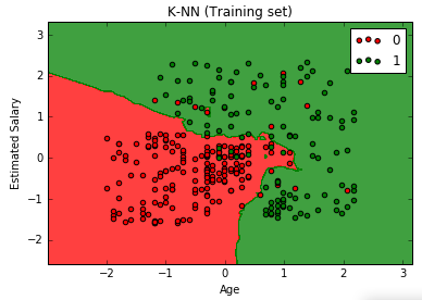

                                               

From the above graph, we can see that KNN is a nonlinear classifier.

Now, we visualize the result for the test set. 

# Visualising the Test set results 
from matplotlib.colors import ListedColormap 
X_set, y_set = X_test, y_test 
X1, X2 = np.meshgrid(np.arange(start = X_set[:, 0].min() - 1, stop = X_set[:, 0].max() + 1, step = 0.01), 
np.arange(start = X_set[:, 1].min() - 1, stop = X_set[:, 1].max() + 1, step = 0.01)) 
plt.contourf(X1, X2, classifier.predict(np.array([X1.ravel(), X2.ravel()]).T).reshape(X1.shape), alpha = 0.75, 
cmap = ListedColormap(('red', 'green'))) 
plt.xlim(X1.min(), X1.max()) 
plt.ylim(X2.min(), X2.max()) 

for i, j in enumerate(np.unique(y_set)): 
    plt.scatter(X_set[y_set == j, 0], X_set[y_set == j, 1], c = ListedColormap(('red', 'green'))(i), label = j) 

plt.title('K-NN (Test set)') 
plt.xlabel('Age') 
plt.ylabel('Estimated Salary') 
plt.legend() plt.show()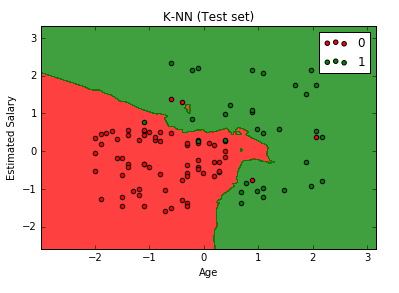

                                             

After executing this code, we can see that these regions are perfectly fitted to the test observation. We can see that the real observation point is in the right region.

Implementing KNN in R

In case you need it, an R version of the Python code above is right below. All the steps as discussed in the Python code have also been exactly done in its R version. Hence, both codes are identical.

# Importing the dataset 
dataset = read.csv('Social_Network_Ads.csv') 
dataset = dataset[3:5] 

# Encoding the target feature as factor dataset
$Purchased = factor(dataset$Purchased, levels = c(0, 1)) 

# Splitting the dataset into the Training set and Test set 
# install.packages('caTools') 
library(caTools) 
set.seed(123) 
split = sample.split(dataset$Purchased, SplitRatio = 0.75) 
training_set = subset(dataset, split == TRUE) 
test_set = subset(dataset, split == FALSE) 

# Feature Scaling 
training_set[-3] = scale(training_set[-3]) 
test_set[-3] = scale(test_set[-3]) 

# Fitting K-NN to the Training set and Predicting the Test set results 
library(class) 
y_pred = knn(train = training_set[, -3], test = test_set[, -3], cl = training_set[, 3], k = 5, prob = TRUE) 

# Making the Confusion Matrix 
cm = table(test_set[, 3], y_pred) 

# Visualising the Training set results 
library(ElemStatLearn) 
set = training_set 
X1 = seq(min(set[, 1]) - 1, max(set[, 1]) + 1, by = 0.01) 
X2 = seq(min(set[, 2]) - 1, max(set[, 2]) + 1, by = 0.01) 
grid_set = expand.grid(X1, X2) 
colnames(grid_set) = c('Age', 'EstimatedSalary') 
y_grid = knn(train = training_set[, -3], test = grid_set, cl = training_set[, 3], k = 5) 
plot(set[, -3], main = 'K-NN (Training set)', xlab = 'Age', ylab = 'Estimated Salary', xlim = range(X1), ylim = range(X2)) 
contour(X1, X2, matrix(as.numeric(y_grid), length(X1), length(X2)), add = TRUE) 
points(grid_set, pch = '.', col = ifelse(y_grid == 1, 'springgreen3', 'tomato')) 
points(set, pch = 21, bg = ifelse(set[, 3] == 1, 'green4', 'red3')) 

# Visualising the Test set results 
library(ElemStatLearn) 
set = test_set 
X1 = seq(min(set[, 1]) - 1, max(set[, 1]) + 1, by = 0.01) 
X2 = seq(min(set[, 2]) - 1, max(set[, 2]) + 1, by = 0.01) 
grid_set = expand.grid(X1, X2) 
colnames(grid_set) = c('Age', 'EstimatedSalary') 
y_grid = knn(train = training_set[, -3], test = grid_set, cl = training_set[, 3], k = 5) 
plot(set[, -3], main = 'K-NN (Test set)', xlab = 'Age', ylab = 'Estimated Salary', xlim = range(X1), ylim = range(X2)) 
contour(X1, X2, matrix(as.numeric(y_grid), length(X1), length(X2)), add = TRUE) 
points(grid_set, pch = '.', col = ifelse(y_grid == 1, 'springgreen3', 'tomato')) 
points(set, pch = 21, bg = ifelse(set[, 3] == 1, 'green4', 'red3'))

Improving the Accuracy of KNN Algorithm

There has been continuous research to find ways to improve a KNN classifier model. Some of the most useful techniques to data are discussed below-

• Using a Different Distance Function The default distance metric in Scikit-Learn for KNN is Minkowski. You should test other distance functions such as cosine similarity or hamming distance and see which one performs better for your model.
• Resolving the Majority Vote Issues KNN algorithm determines the class of new data by performing a simple majority vote system. This approach sometimes ignores the similarities among data and allows the occurrence of a double classification class that can lead to misclassification. This majority vote issue can be resolved by calculating the distance weight using a combination of the local mean based k-nearest neighbor(LMKNN) and distance weight k-nearest neighbor(DWKNN). I suggest you read this amazing paper on this method.
• Adjusting Weights of the Features In this method, a certain weight is allocated to different features based on their importance. The features now have different effects on the classification procedure of the model and eventually avoiding the deviation of a classification process due to the assumption of the same effect of each feature. Hence, it improves the accuracy of the model.
• Using Hybrid Algorithms Using other methods alongside with KNN. This approach makes the models more robust and powerful. A popular algorithm is SV-kNNC. It consists of three steps. First, Support Vector Machines(SVMs) are used to select some important training data. Then, K-means Clustering is applied to assign the weight to each training instance. Finally, unseen examples are classified by KNN.
• Using Tolerant Rough Set Tolerant rough relation can be related to object similarity. Two objects are called similar if and only if they satisfy the requirements of the tolerant rough relation. Using a tolerant rough set, objects are selected from the training data and similarity functions are constructed. A genetic algorithm is used to find optimal similarity metrics. This research paper shows us how to apply the method.

How to Avoid Overfitting in KNN?

Actually KNN reduces the risk of overfitting. But this can be done when the value of K is chosen optimally. If we choose a small value of K for a large data set, we are still at the risk to overfit the model. There are chances that it would introduce noise to the model. Hence, leading to overfitting the model and performance degradation on prediction,

Taking a large value would also pose threats to the model i.e. it would smoothen things up so much that the model may miss important details about the classes. In our above example, if we choose K to be equal to the number of training instances, and there are more green data points than red, then the whole distribution will be taken as blue!

So, we have to be wise while choosing the value for K. It should be large enough to avoid allowing noise and small enough not to be biased. This can be done by hyperparameter tuning with the help of Grid Search techniques.

Pros and Cons of KNN

We have already implemented the algorithm above and we are now fully aware of the usability of this algorithm. But before making it our go-to the algorithm in production, we must check and balance the advantages and disadvantages of KNN.

Pros

• Simple KNN is a very intuitive algorithm, making it simple and easy to implement.
• No Training Time Being an instance-based algorithm, KNN requires no training to make predictions.
• No Assumptions of Data KNN do not assume any characteristics of the data to make predictions. All it needs a set of data and it will just be there waiting to predict the unknowns.
• Adaptive to Change As it makes prediction without a training step involved, it is adaptive to change in data. You can seamlessly add new data to the model without affecting the prediction compatibility of the model.
• Inherently Multiclass Many classification algorithms e.g. SVM are binary in nature. Implementing multiclass classification with those classifier tasks would require extra effort. But KNN is inherently capable to work with multiclass problems.

Cons

• Slow Since KNN makes all the predictions without a training stage, it has to calculate all the neighbors separately for each unknown data point. When you use KNN with large data sets, the situation gets worse, taking a long time to make each prediction.
• Sensitive to Outliers Since KNN uses distance metrics to determine the class of a new data instance, outliers will badly affect the model accuracy.
• Can not Deal with Missing Data KNN has no inherent capability of handling missing values. If the data set contains missing values, the model will not be able to make predictions.
• Bad with High Dimensions When the data set contains a large number of features, it becomes hard for KNN to calculate distances in each dimension. This eventually degrades the performance of your model.
• Not Suited for Imbalanced Data As the algorithm is based on distance metrics, it does not perform well on imbalanced data. When there is two class with one class having more data points than the other, the algorithm may get biased to the larger class of data.

Final Thoughts

In the tutorial, I have tried to discuss all the key aspects of the k nearest neighbor algorithm. In summary, the key take ways are-

• What KNN algorithm is and how it works
• Features of KNN algorithm
• Choosing the distance metric and the value of K
• Implementation of the algorithm in both Python and R
• Pros and Cons of KNN

I hope this tutorial helped you to understand all those concepts well. I admit your suggestions and opinions about the tutorial to make it more worthy. Please share your thoughts with me.

Happy Machine Learning!