Polynomial Regression in Two Minutes (with Python Code) | Machine Learning

If you have worked with linear regression models such as simple linear regression or multiple linear regression, you might have observed some drawbacks of those models. It is not like that the models are bad, rather it is due to the underlying property of your data. You see, data can take different shapes. And you need to use the right kind of algorithm to make the best predictive model out of your data.

In this tutorial, we are going to understand a different type of regression algorithm, the Polynomial Regression. After discussing the concepts, we will build a predictive model with the algorithm in Python. Let's dive into that!

What is Polynomial Regression?

Polynomial regression is a form of regression analysis in which the relationship between the independent variable x and dependent variable y is modeled as an nth degree polynomial of x. That is, if your dataset holds the characteristic of being curved when plotted in the graph, then you should go with a polynomial regression model instead of Simple or Multiple Linear regression models.

The equation for Polynomial Regression looks very similar to that of Multiple Linear Regression.

y=b0+b1*x1+b2*(x1)2+....+bn*(x1)n

The main difference is that in Multiple Linear Regression, there are several variables of the same degree but here the single variable has different powers. 

Why Polynomial Regression?

Let's say you have a dataset and fit both Simple and Polynomial Regression to that data.

                                                                      Plotted with a linear regression model

 

Here you can see the data has a tendency to grow in a non-linear fashion. Hence a simple linear model could not find the most optimal line that can fit the data well and has a very poor accuracy level.

  

                                                                 Plotted with a polynomial regression model

Now if you look at the polynomial regression, you will clearly see the difference. The Polynomial model has fitted the dataset well with a higher accuracy rate than that of a simple linear model.

There are many cases where you will find great uses of polynomial regression. For example, if you want to discover how diseases spread, how a pandemic or epidemic spread over a continent, and so on. It completely depends on your data. And based on the non-linear characteristics of your data, you should use polynomial regression.

Implementing Polynomial Regression in Python

Now we will jump into a dataset and implement the above idea.

Suppose we have a dataset(Salary_data.csv) that contains the salaries of employees of different positions based on their Level. Let's have a look at the dataset.

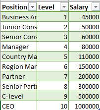
You can download the dataset from here.

If we plot the above data in a graph, it would look like this-

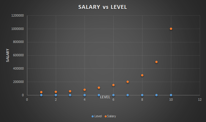
Here, you can observe that our data has a tendency of growing non-linearly. So we are required to use a Polynomial Regression for this case.

The dataset contains just three columns. We will take the second column, Level as our independent variable in the feature matrix, X and the Salary column as the dependent variable in the dependent variable vector, y.

We start by preprocessing the data. You will get the full code in Google Colab. For this use the following codes-

# Polynomial Regression 
# Importing the Essential Libraries 
import numpy as np 
import matplotlib.pyplot as plt 
import pandas as pd 

# Importing the dataset 
dataset = pd.read_csv('Position_Salaries.csv') 
X = dataset.iloc[:, 1:2].values 
y = dataset.iloc[:, 2].values

We skip the splitting part as the dataset contains only 10 values. So let's fit polynomial regression to our whole dataset and for this, you should write the following code-

# Fitting Polynomial Regression to the dataset 
from sklearn.preprocessing import PolynomialFeatures 
from sklearn.linear_model import LinearRegression
poly_reg = PolynomialFeatures(degree = 4) 
X_poly = poly_reg.fit_transform(X) 
poly_reg.fit(X_poly, y) 
lin_reg_2 = LinearRegression() 
lin_reg_2.fit(X_poly, y)

Note: Here, I used degree = 4, you should try with different values for this parameter and watch how your model works. For this dataset, a value of degree 4 just works fine!

Well, we have fitted our model to the dataset. Now, it's time to plot and see how it works.

# Visualising the Polynomial Regression results 
X_grid = np.arange(min(X), max(X), 0.1) 
X_grid = X_grid.reshape((len(X_grid), 1)) 
plt.scatter(X, y, color = 'red') 
plt.plot(X_grid, lin_reg_2.predict(poly_reg.fit_transform(X_grid)), color = 'blue') 
plt.title('Truth or Bluff (Polynomial Regression)') 
plt.xlabel('Position level') 
plt.ylabel('Salary') 
plt.show()

The plot should look like this-

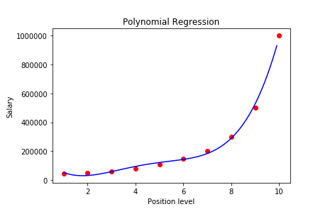
With a 4-degree polynomial regression, we obtained a model that has closely predicted the Salary values. If we used a simple linear regression instead, we could not obtain this level of accuracy.

So now we can use our model to learn how it predicts for an unknown value.

# Predicting an unknown value with Polynomial Regression model y_pred = lin_reg_2.predict(poly_reg.fit_transform([[6.5]]))

For a level value of 6.5, it predicts: 158862

We put the same dataset in a simple linear regression model. And for the same level value of 6.5, it gave us the outcome: 330378.78!

If you compare both the value with the first SALARY vs LEVEL graph, you can understand that our polynomial model has predicted a way better than that of a simple linear regression model.

How to Choose the Correct Degree of Polynomial for the Regression Model? 

There is no "exact" way to choose the right value for the degree of a polynomial regression model. You can start with an initial value then continuously increase(or decrease) the values and check whether the curve fits your model more perfectly than the past one.

This process usually is not a good solution because it is hard to make this working every time i.e. think about a million-degree polynomial. This process will be time-consuming and complex which will not worth the effort. Because of the issue with overfitting.

When you are optimizing the polynomial equation to perfectly describe your data, you are making the model prone to overfitting. If you use this predictive model on unseen data, the performance will fall down in contrast to the training period. And this is not desirable for your model.

Cross-validation can be handy to solve this problem. You can check a set of polynomial values with cross-validation. Then take the value which provided the best performance on average. This will prevent your model to overfit during the training stage. Although we are fitting a nonlinear model to the data, it is still a linear model. This is because the regression function takes into account the parameters, not the covariates(the number of degrees)

Is Polynomial Regression Linear or Non-Linear?

Although we are fitting a nonlinear model to the data, it is still a linear model. This is because the regression function takes into account the parameters, not the covariates(the number of degrees).

You can make any transformation to the variables, but still, the statistical estimation problem is linear.

For this, the polynomial variation is not considered as a different regression model. It is just a special case of multiple linear regression. 

Final Words

In this tutorial, I have tried to discuss all the concepts of polynomial regression. The key take ways from the tutorial are-

• What polynomial regression is and how it works
• Implementing polynomial regression in Python
• how to choose the best value for the degree of the polynomial

Hope this tutorial has helped you to understand all the concepts. If you have any questions, please let me know in the comments. 

Happy Machine Learning!