Artificial Neural Networks | Machine Learning

In this article, we are going to learn and implement an Artificial Neural Network(ANN) in Python.

Artificial Neural Network: An artificial neural network (ANN), usually called a neural network" (NN) is a mathematical model or computational model that tries to simulate the structure and functional aspects of biological neural networks. It consists of an interconnected group of artificial neurons and processes information using a  connectionist approach to computation.

To get a clear idea, let's take a look at a biological neuron.

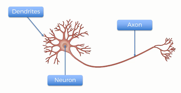
A human neuron has three parts- the main body, the axon, and the dendrites. Though one neuron itself does not have any significance, when millions or probably billions of neurons work together, they can process a task like reading and understanding this article. 

Well, you can think of an artificial neuron as a simulation of a human neuron. It tries to mimic the works of a human neuron using mathematics and machine learning algorithms. Here is also, as a biological neuron, a single AN can not do any significant task. But when we connect a number of neurons in layers, they together can do some tasks like classification or regression.

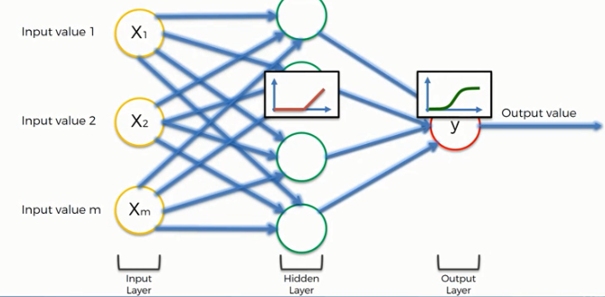
Here you can see a simplified illustration of an artificial neuron. It takes inputs from some neurons i.e. x1, x2, xm, processes them using some mathematical functions called activation functions and produces an output. ANN has much more complex structures. It also includes some hidden layers and other structures.

Activation Functions: An activation function directs the output of a neuron or node, which means after receiving a set of inputs, it chooses what will be the output of that neuron. Depending on the kind of activation function, the output of a neuron varies. There are various types of activation functions. But these four are prominent ones.

• Threshold Function: This is the most basic type of activation function. It simply outputs a yes/no type of value. When the weighted sum is(the sum of weighted input from the input layers) less than zero, it simply provides 0, and when the weighted sum is greater or equals to zero, it provides
• Sigmoid Function: This is one of the most used activation functions. It provides a continuous output. If the input value is less than zero its output will be zero. For a value zero or greater than zero it provides a continuous output value ranges between zero and one. It is a useful function for tasks like regressions. It is usually used in the output node.
• Rectifier Function: It is one of the most popular activation functions. It provides a zero for a negative value and gradually increases to one for a positive value. It is widely used in the input layer nodes.
• Hyperbolic tangent function: It provides output for both negative and positive input values.

How Does the Neural Network Work?

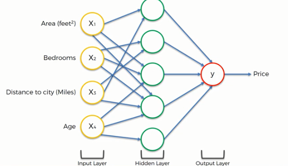
When we connect a number of artificial neurons, that forms a neural network. Then the network can carry out some tasks like classification and regression. To understand the whole idea, let's take an example, assume that we need to find the price of an apartment in a particular area, where the input parameters are the area of the apartment, number of bedrooms, how far it is from the city, and the age of the apartment. Now let's build an ANN model that will predict the price of a particular apartment using this set of input parameters. We are not going into the details, but assume that in the hidden layer we are using an activation function i.e. Rectifier function that calculates the weighted input and pass a value to the output layer where we are using another activation function i.e. Sigmoid function, that upon the input from the hidden layer, calculates the probable value of that apartment. Here we have shown a simplified feedforward network, you may need to use more complex models for other problems.

How do Neural Networks Learn?

Though the idea of learning neural networks is a bit complex, we can simplify the concept. In a simple sense, we feed in inputs to the input layer nodes(individual neurons), which are connected to some hidden layer nodes. The inputs are processed and fed to the output layer. Then we compare the predicted value with the actual value using a cost function. In ML,  a cost function is used to measure how good or bad a model is performing. Here we take a cost function, C which is the squared average difference between the predicted and actual outcomes.

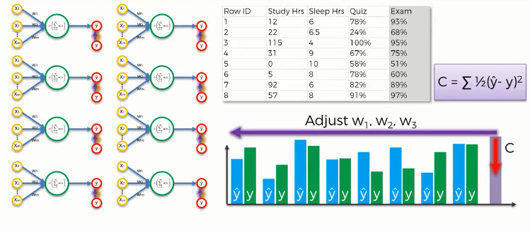
Then we update the weights in the input layer based on the cost function output. This update is performed by using a gradient descent function. This type of network is called a backpropagation network. Because we are providing the input and updating the weights from the output iteratively. 

After some iterations (until a satisfactory outcome), we assume that the model has learned successfully.

Gradient Descent Function

Gradient descent is an optimization algorithm for updating the weights to the input layer nodes after the comparison done by the cost function. It uses a first-order differential equation that tries to minimize the cost function. That means it tries to find the lowest error value.

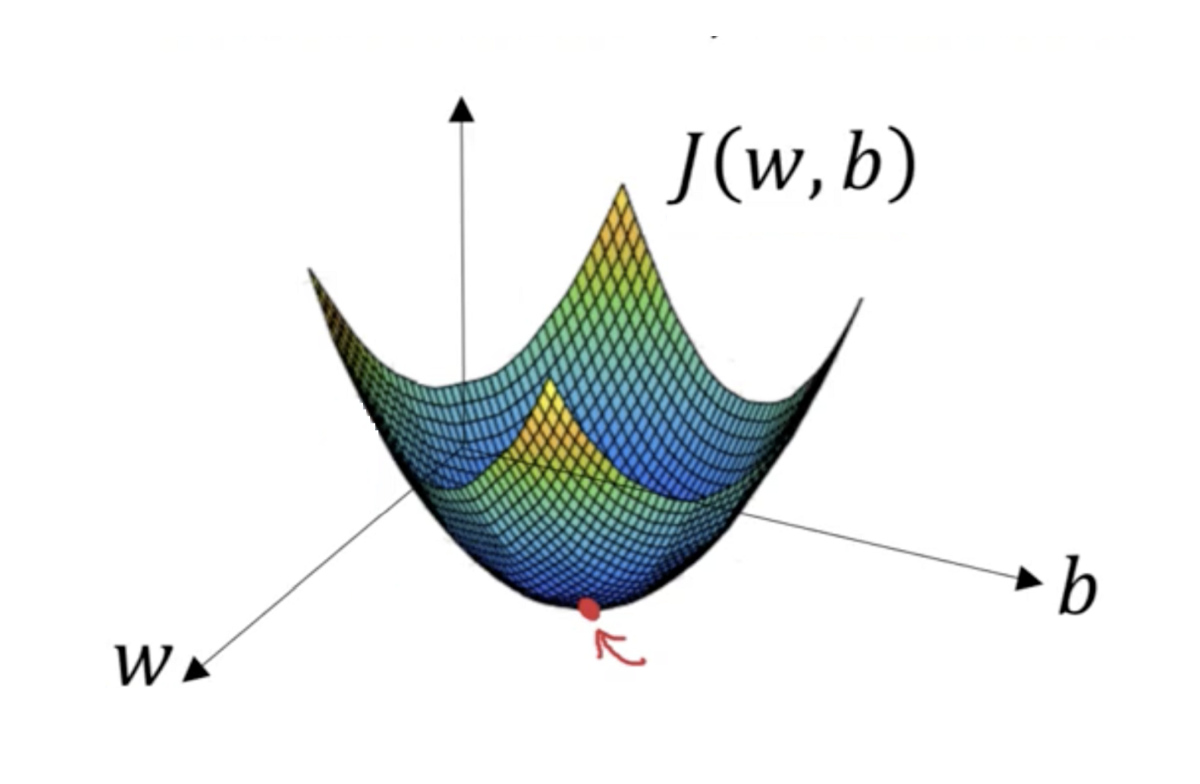
There are various types of gradient descent functions. Among them, the Batch gradient descent function (shown above) and Stochastic gradient descent function are most commonly used.

The stochastic gradient descent function is more optimized than the Batch gradient function as it can avoid the local minimum. Local minimum happens when the gradient function finds a minimum error value that seems fine initially. But if the function could go further it would find the best minimum error value.

In this article, we will use the stochastic gradient descent function. 

Let's understand the steps required to train a model with Stochastic gradient Descent 

STEP 1: Randomly initialize the weights to small numbers close to 0 (but not 0). 

STEP 2: Input the first observation of your dataset in the input layer, each feature in one input node. 

STEP 3: Forward-propagation: From left to right, the neurons are activated in a way that the impact of each neuron's activation is limited by the weights. Propagate the activations until getting the predicted result y. 

STEP 4: Compare the predicted result to the actual result. Measure the generated error. 

STEP 5: Back-propagation: from right to left, the error is back-propagated. Update the weights according to how much they are responsible for the error. The learning rate is decided by how much we update the weights. 

STEP 6: Repeat Steps 1 to 5 and update the weights after each observation (Reinforcement Learning). Or: Repeat Steps 1 to 5 but update the weights only after a batch of observations (Batch Learning). 

STEP 7: When the whole training set passes through the ANN, that makes an epoch. Redo more epochs.

ANN in Python: In this tutorial, we are going to implement an artificial neural network in Python. 

We have a dataset of a bank containing the transaction data of customers. Let's have a look at the dataset-

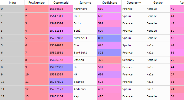
You can download the whole dataset from here.

The dataset contains a number of different features. Now, using these features of the dataset, our task is to classify whether a customer stays or departs from the bank. So this is a classification problem.

For building neural networks we need libraries and modules like Keras, Theona, and TensorFlow. Ensure that you have properly installed them in your Anaconda environment. You can find the guidelines for installing these here. You will get the code in Google Colab also.

First of all, we will import some essential libraries. 

# Importing the libraries
import numpy as np
import pandas as pd
import tensorflow as tf

In the dataset, the last column Exited represents the state of a customer(stays or leaves) and is the only dependent variable. So we will take this column in the dependent variable vector. The rest of the columns are independent, so we will take all except the first three columns into the feature matrix.

# Importing the dataset
dataset = pd.read_csv('Churn_Modelling.csv')
X = dataset.iloc[:, 3:-1].values
y = dataset.iloc[:, -1].values

Here some of the features are categorical variables. So we will encode them.

# Encoding categorical data
# Label Encoding the "Gender" column
from sklearn.preprocessing import LabelEncoder
le = LabelEncoder()
X[:, 2] = le.fit_transform(X[:, 2])

# One Hot Encoding the "Geography" column
from sklearn.compose import ColumnTransformer
from sklearn.preprocessing import OneHotEncoder
ct = ColumnTransformer(transformers=[('encoder', OneHotEncoder(), [1])], remainder='passthrough')
X = np.array(ct.fit_transform(X))

Now we split the dataset into training and test sets.

# Splitting the dataset into the Training set and Test set
from sklearn.model_selection import train_test_split
X_train, X_test, y_train, y_test = train_test_split(X, y, test_size = 0.2, random_state = 0)

# Feature Scaling
from sklearn.preprocessing import StandardScaler
sc = StandardScaler()
X_train = sc.fit_transform(X_train)
X_test = sc.transform(X_test)

Now, we have come to the main part of our program. We will build a neural network using the Keras library.

# Importing the Keras libraries and packages
import keras
from keras.models import Sequential
from keras.layers import Dense

We will initialize the ANN using the Sequential class from Keras.

# Initialising the ANN
ann = tf.keras.models.Sequential()

Now, we will add the hidden layer. The dataset contains eleven independent variables. It is a rule of thumb that we take half of the dependent variable in the hidden layer. So the units parameter is set to 6. Here we used the rectifier functions as the activation function.

# Adding the input layer and the first hidden layer
ann.add(tf.keras.layers.Dense(units=6, activation='relu'))

 We can add more than one hidden layer to our network.

# Adding the second hidden layer
ann.add(tf.keras.layers.Dense(units=6, activation='relu'))

Now, we will add the output layer. Here, we have only one dependent variable. So our output layer only contains one node. We used the sigmoid function as the activation function.

# Adding the output layer
ann.add(tf.keras.layers.Dense(units=1, activation='sigmoid'))

 Let's compile the whole ANN before starting to run. Here we use the stochastic gradient descent function as the optimizer. adam is one of the most used stochastic gradient descent functions. We choose binary_crossentropy as the loss function as this is a binary classification problem.

# Compiling the ANN
ann.compile(optimizer = 'adam', loss = 'binary_crossentropy', metrics = ['accuracy'])

It's time to fit the classifier algorithm into our dataset. we take the number of iteration, nb_epoch to 100 which means the whole network will run a hundred times.

# Fitting the ANN to the Training set
ann.fit(X_train, y_train, batch_size = 32, epochs = 100)

y_pred = ann.predict(X_test)
y_pred = (y_pred > 0.5)
print(np.concatenate((y_pred.reshape(len(y_pred),1), y_test.reshape(len(y_test),1)),1))

Let's see how good our model is for making the prediction.

from sklearn.metrics import confusion_matrix, accuracy_score
cm = confusion_matrix(y_test, y_pred)
ac = accuracy_score(y_test, y_pred)
print(cm)
print(ac)

From the above confusion matrix, we can see the accuracy of the model is 84%.