- An Introduction to Machine Learning | The Complete Guide
- Data Preprocessing for Machine Learning | Apply All the Steps in Python
- Regression
- Learn Simple Linear Regression in the Hard Way(with Python Code)
- Multiple Linear Regression in Python (The Ultimate Guide)
- Polynomial Regression in Two Minutes (with Python Code)
- Support Vector Regression Made Easy(with Python Code)
- Decision Tree Regression Made Easy (with Python Code)
- Random Forest Regression in 4 Steps(with Python Code)
- 4 Best Metrics for Evaluating Regression Model Performance
- Classification
- A Beginners Guide to Logistic Regression(with Example Python Code)
- K-Nearest Neighbor in 4 Steps(Code with Python & R)
- Support Vector Machine(SVM) Made Easy with Python
- Kernel SVM for Dummies(with Python Code)
- Naive Bayes Classification Just in 3 Steps(with Python Code)
- Decision Tree Classification for Dummies(with Python Code)
- Random forest Classification
- Evaluating Classification Model performance
- A Simple Explanation of K-means Clustering in Python
- Hierarchical Clustering
- Association Rule Learning | Apriori
- Eclat Intuition
- Reinforcement Learning in Machine Learning
- Upper Confidence Bound (UCB) Algorithm: Solving the Multi-Armed Bandit Problem
- Thompson Sampling Intuition
- Artificial Neural Networks
- Natural Language Processing
- Deep Learning
- Principal Component Analysis
- Linear Discriminant Analysis (LDA)
- Kernel PCA
- Model Selection & Boosting
- K-fold Cross Validation in Python | Master this State of the Art Model Evaluation Technique
- XGBoost
- Convolution Neural Network
- Dimensionality Reduction
Data Preprocessing for Machine Learning | Apply All the Steps in Python | Machine Learning

Data Preprocessing: Data Prepossessing is the first stage of building a machine learning model. It involves transforming raw data into an understandable format for analysis by a machine learning model. It is a crucial stage and should be done properly. A well-prepared dataset will give the best prediction by the model.
Why Data Preprocessing is so Important?
- Raw data may contain improper values or in an incorrect format.
- Making the dataset feasible for the analysis.
- For achieving the best result from a dataset.
- Quality result depends on quality data. I.e. improper or missing data can lead a model to give confusing output
Major tasks in Data Preprocessing: The major tasks in Data Preprocessing are given below:
1.Data cleaning: Fill in missing values, smooth noisy data, identify or remove outliers, and resolve inconsistencies.
2.Data Integration: Integration of multiple databases, data cubes, or files.
3.Data Transformation: Normalization and aggregation.
4.Data reduction: Reduced representation in volume but produces the same or similar analytical results.
5.Data discretization: Part of data reduction but with particular importance, especially for numerical data.
Important: We will use the Spyder IDE from Anaconda for executing the codes. To start with executing the following codes in Spyder, first, you need to set the folder where you keep this dataset as the working directory. To do so, you need to go to the file explorer of your Spyder IDE and set the folder as the working directory.
.jpg)
Then for executing the code given here, you need to write them on the Spyder editor. After that, you need to select all the code and press ctrl+enter(in windows). Then you will see the output on the IPython console.
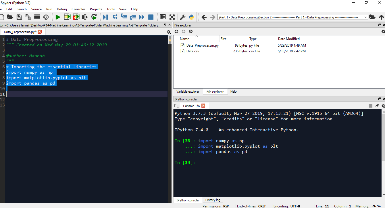
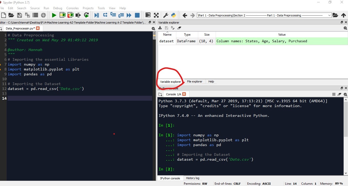
You can see the variables from the variable explorer.
In this tutorial, I will show you how to pre-process your data using several techniques.
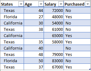
Getting the Dataset: There are several places from where you can download standard datasets. Kaggle is the best place for that. You can also get data from UCI machine learning database, data.gov, and google public dataset. For this tutorial, I used this dataset named Data.csv.
You can download it from here.
Importing the Libraries: Libraries are tools in python that we can use to make a specific job. And what's cool about these libraries is that you just have to give some inputs and the library will do the rest of the job. For making our models we are going to use a lot of libraries but there are three most common libraries that are used in every program. So, first of all, we will import those libraries. You will get the full code in Google Colab. Now let's get into the work.
import numpy as np
import matplotlib.pyplot as plt
import pandas as pd
Here, the library numpy contains lots of predefined tools to do mathematical and scientific operations on the data. matpolotlib.pyplot is the library to plot the data in charts. And the last one, pandas provides tools to read and import the dataset.
Importing the Dataset: First, we import the dataset from our working directory. For this, we need to do the following:
dataset = pd.read_csv('Data.csv') Note: The dataset must be in CSV format.
There is something you must understand in machine learning is that in Python, we need to distinguish the matrix of feature and the dependent variable vector in our dataset. The independent variables which are used to predict the value of the dependent variable are contained in the Feature Matrix. The dependent variable is kept in the dependent variable vector. If you look back into the dataset you can see that the first three columns- States, Age, Salary are independent variables that we must take in the feature matrix. Let's denote it as X. And then we take the Purchased column in the dependent variable matrix, denoting y. The codes are as follows:
X = dataset.iloc[:, [0,1,2]].values y = dataset.iloc[:, 3].values
The output for X should be like this:
array([['Texas', 44.0, 72000.0],
 ['Florida', 27.0, 48000.0],
 ['California', 30.0, 54000.0],
 ['Texas', 38.0, 61000.0],
 ['California', nan, 65000.0],
 ['Texas', 35.0, 58000.0],
 ['California', 40.0, nan],
 ['Texas', 48.0, 79000.0],
 ['Florida', 50.0, 83000.0],
 ['Texas', 37.0, 67000.0]], dtype=object)
And for y it will be:
array(['No', 'Yes', 'No', 'No', 'Yes', 'Yes', 'No', 'Yes', 'No', 'Yes'], dtype=object)
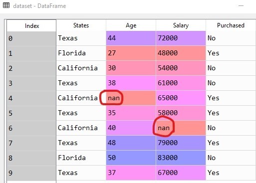
Handle the Missing Data: If you look into the dataset you should find that there are some missing values in age and salary columns(actually it's two, one in the Age column and another in the Salary column). This missing data will cause irregularities in our machine learning model. So we need to handle these missing data. For this, we use SimpleImputer class from the Scikit-learn library of Python. There are many strategies to handle missing data, we can take the average or median or mean of the column. Here we will take the median value.
Handling the missing values
from sklearn.impute import SimpleImputer imputer = SimpleImputer(missing_values=np.nan, strategy='mean') imputer.fit(X[:, 1:3]) X[:, 1:3] = imputer.transform(X[:, 1:3])
Note: Python uses 'NaN' to represent missing values.
The output should look like this:
array([['Texas', 44.0, 72000.0], ['Florida', 27.0, 48000.0], ['California', 30.0, 54000.0], ['Texas', 38.0, 61000.0], ['California', 38.77777777777778, 65000.0], ['Texas', 35.0, 58000.0], ['California', 40.0, 65222.22222222222], ['Texas', 48.0, 79000.0], ['Florida', 50.0, 83000.0], ['Texas', 37.0, 67000.0]], dtype=object)
Here the missing values are replaced by the mean of the respective column values(highlighted in yellow).
Categorical Data: In our dataset, we have two columns- States and Purchased, both containing categorical data. These two variables are categorical variables because simply they contain categories(i.e. name of a state, or yes/no values). Since machine learning models are based on mathematical equations, you can intuitively understand that they would not fit in our model well. So, we can not keep the categorical variables because we only can use numbers in the equations.
That's why we need to encode the categorical variables.
#Encoding the categorical variables from sklearn.preprocessing import LabelEncoder, OneHotEncoder from sklearn.compose import ColumnTransformer labelencoder_X = LabelEncoder() X[:, 0] = labelencoder_X.fit_transform(X[:, 0]) labelencoder_y = LabelEncoder() y = labelencoder_y.fit_transform(y) y = y.reshape(-1, 1)
Note: here, LabelEncoder converts the categorical values into numbers so that they could be used in the machine learning equation.
The outputs are-
For X:
array([[2, 44.0, 72000.0], [1, 27.0, 48000.0], [0, 30.0, 54000.0], [2, 38.0, 61000.0], [0, 38.77777777777778, 65000.0], [2, 35.0, 58000.0], [0, 40.0, 65222.22222222222], [2, 48.0, 79000.0], [1, 50.0, 83000.0], [2, 37.0, 67000.0]], dtype=object)
For y:
array([0, 1, 0, 0, 1, 1, 0, 1, 0, 1])
At the output, for X the values for the States column and for y, the values for the Purchased column are replaced by numbers.
Note: Though categorical values are converted to numbers, they will still cause a problem. You can observe that the encoding has made one state having a higher or lower value than others. As a machine learning model is based on equations, the numbers denoting the states will have some effect on the equation(i.e. persons from a higher/lower value state may be predicted to have a higher/lower salary than persons from other states). But this is not the thing we wanted, these are actually categorical data with no relational order between them. To solve this problem, we need to make dummy variables so that our machine learning model does not confuse with the weight of the categorical values. The following code will generate a dummy variable for each of the three states contained in our dataset.
#Creating dummy variables for the encoded categorical values transformer = ColumnTransformer([('one_hot_encoder', OneHotEncoder(), [0])],remainder='passthrough') X = np.array(transformer.fit_transform(X), dtype=np.float) After creating dummy variables the X dataset should look like:
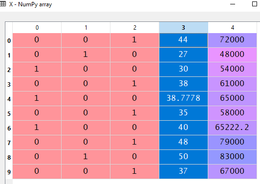
Here columns 0, 1, and 2 represent dummy variables for the three categorical values.
We need not make dummy variables for y dataset. Since this is the dependent variable and our machine learning model knows it is a category and that there is no order between the two(yes/no) values. So, LabelEncoder will do good enough for the y dataset.
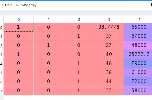
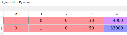
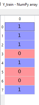
Splitting the dataset: Now, we need to split the dataset into training and test dataset. The training dataset is used to train the machine learning model and the test dataset is to test the model.
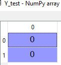
#Splitting the datasets from sklearn.model_selection import train_test_split X_train, X_test, y_train, y_test = train_test_split(X, y, test_size = 0.2, random_state = 0 )
Note: Here, test_size = 0.2 means we take 20% of our data to the test set, and the remaining 80% will be in the training set. random_state = 0 is to ensure that after splitting, your datasets and our dataset look become the same.
After splitting the dataset should look like this:
Feature Scaling: Now, we come to the last part of preprocessing. Let's explain what is features scaling and why we need to do it.
If you look at the dataset again, you can see the two columns namely Age and Salary contain numerical data. You should notice that the variables are not on the same scale. The Age is going from 27 to 50 while the Salary has a range of 48000 to 83000. And there is no distinguished linear relationship between these two columns. This will cause inaccurate predictions by our model. So we need to scale them to get a more accurate prediction from the model.
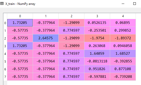
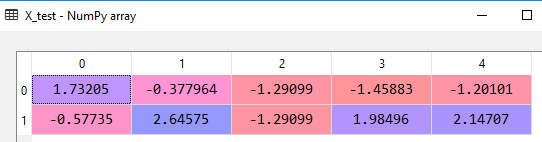
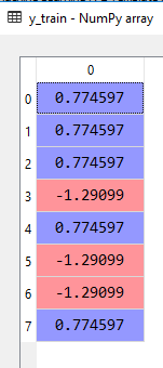
# Feature Scaling from sklearn.preprocessing import StandardScaler sc_X = StandardScaler() X_train = sc_X.fit_transform(X_train) X_test = sc_X.transform(X_test) sc_y = StandardScaler() y_train = sc_y.fit_transform(y_train)
After feature scaling the dataset will look like the following:
Data preprocessing is the fundamental step to start creating a model, we will go further and see how the machine learning model is built using various algorithms and techniques in the following articles.