Decision Tree Classification for Dummies(with Python Code) | Machine Learning

In this article, we are going to understand the concept of Decision Tree algorithm for classification and then we will implement it in Python.

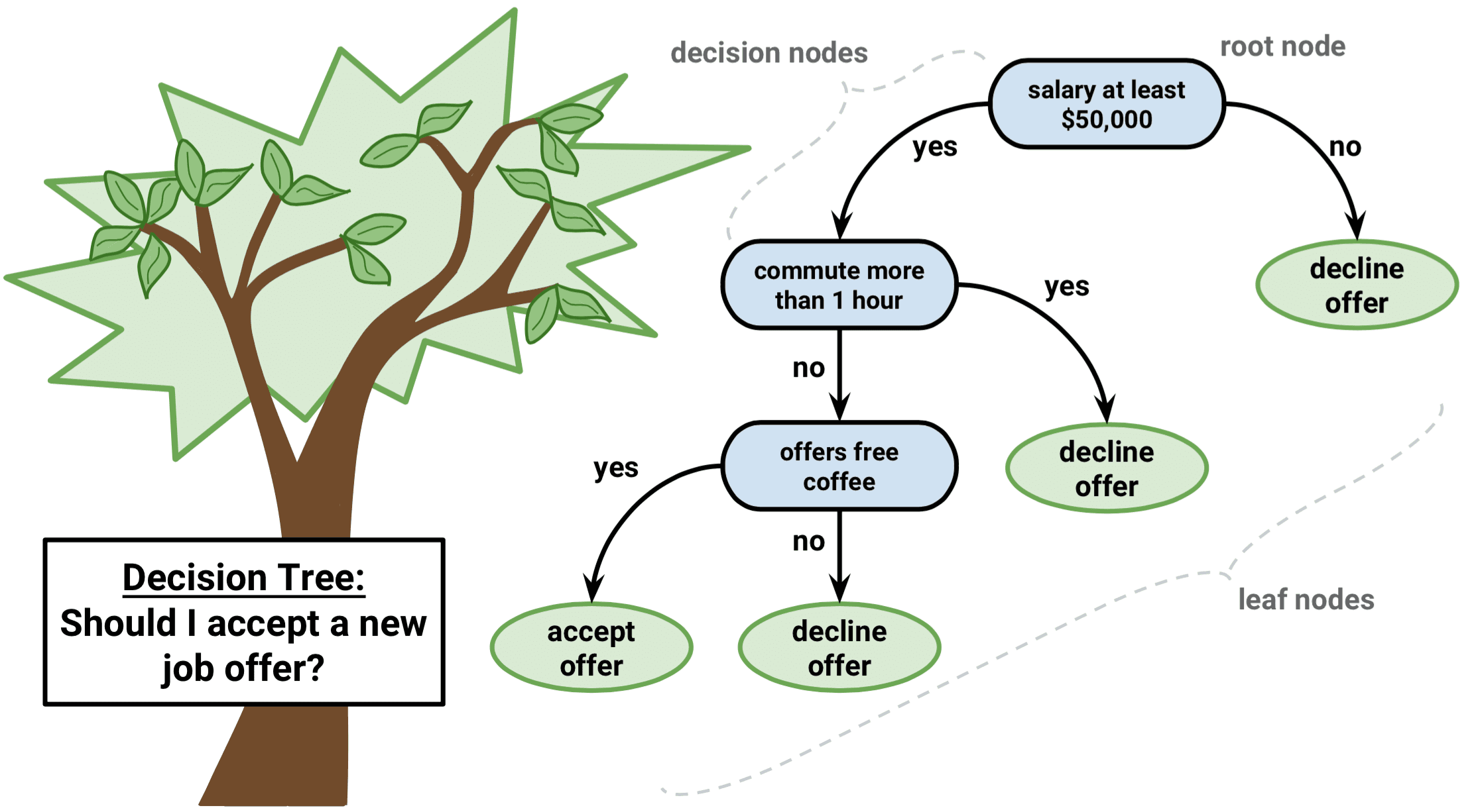
Decision Tree Classification: This Classification is based on the decision tree structure. A decision tree is a form of a tree or hierarchical structure that breaks down a dataset into smaller and smaller subsets. At the same time, an associated decision tree is incrementally developed. The tree contains decision nodes and leaf nodes. The decision nodes are those nodes represent the value of the input variable(x). It has two or more than two branches. The leaf nodes contain the decision or the output variable(y). The decision node that corresponds to the best predictor becomes the topmost node and called the root node.

When You Should Choose a Decision Tree?

Assume you have a dataset where the data points are randomly distributed. Consider the following illustration.

                  

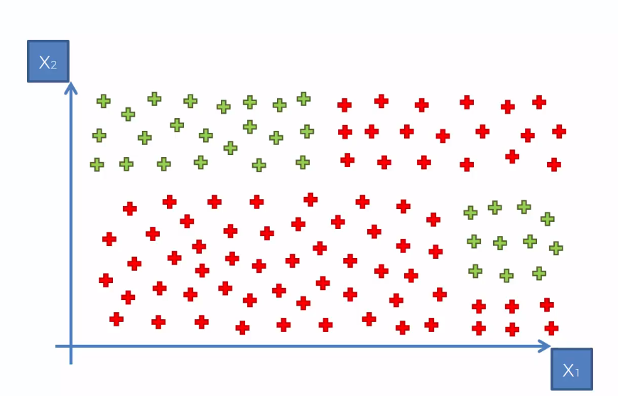
For a randomly distributed dataset like this, you should not go for the other classification algorithm like SVM, K-means, or Naive Bayes. As more randomness in data will create more entropy, you must choose an algorithm that minimizes the entropy and maximize the information gain. In that context, you should implement a Decision Tree for classification.

Entropy is the measure of randomness or impurity contained in a dataset. Information gain is the opposite of entropy that measures the decrease in entropy.

How does the Algorithm Work?

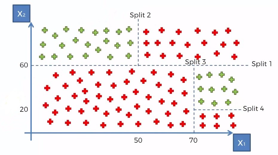
This algorithm works based on maximizing the information gain in the groups of data points. That means it splits the data points into optimal parts(subtree) in such a way that it contains as much as information and less randomness. It selects the best attributes using the Attribute Selection Measures to split the data. For the above data points, it would split them in the following way.

           

Then it makes the attribute a decision node and breaks the dataset into smaller subsets(subtree). It repeats the process recursively for each child node until there is no more remaining attributes or no more instances to add to the tree.

For the above dataset, it will make a tree like this.

                     

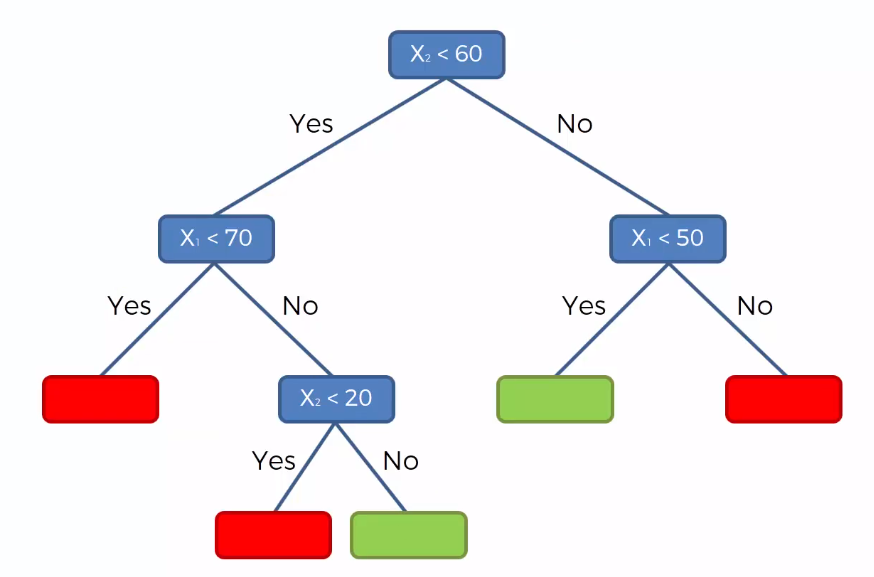
Then to classify a new data point, it will traverse the tree and try to match that point to one of the decision nodes. If it reaches that node, it returns the leaf node value for that data point.

It is quite a simple method but at the same time, it lies in the foundation of some of the more modern and powerful method of machine learning.

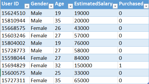
Decision Tree Classification in python: Now, we will implement the above algorithm in Python. For this task, we will use Social_Network_Ads.csv dataset. Lets have a glimpse of that dataset.

                                                          o

 You can download the whole dataset from here.

First of all, we will import the libraries. You will get the full code in Google Colab also.

import numpy as np
import matplotlib.pyplot as plt
import pandas as pd

Then we will import the dataset into our program and divide the attributes into Feature matrix and dependent variable vectors. Here the Age and EstimatedSalary are the independent attributes, so we will put them into the Feature matrix and the Purchased column into the dependent variable vector.

# Importing the dataset
dataset = pd.read_csv('Social_Network_Ads.csv')
X = dataset.iloc[:, [2, 3]].values
y = dataset.iloc[:, 4].values

Now, we will split the dataset into training and test sets.

# Splitting the dataset into the Training set and Test set
from sklearn.model_selection import train_test_split
X_train, X_test, y_train, y_test = train_test_split(X, y, test_size = 0.25, random_state = 0)

We need to scale our dataset for a more accurate prediction.

# Feature Scaling
from sklearn.preprocessing import StandardScaler
sc = StandardScaler()
X_train = sc.fit_transform(X_train)
X_test = sc.transform(X_test)

It's time to fit the Decision tree algorithm to our dataset.

# Fitting Decision Tree Classification to the Training set
from sklearn.tree import DecisionTreeClassifier
classifier = DecisionTreeClassifier(criterion = 'entropy', random_state = 0)
classifier.fit(X_train, y_train)

Note: Here criterion is the parameter that measures the quality of a split. We choose 'entropy' for the information gain.

We have built our model. Now, we will predict the result.

# Predicting the Test set results
y_pred = classifier.predict(X_test)

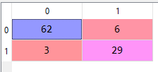
To learn how our model performed on the dataset, we will build a confusion matrix.

# Making the Confusion Matrix
from sklearn.metrics import confusion_matrix
cm = confusion_matrix(y_test, y_pred)

After executing, the output of the confusion matrix would look like this.

                                                                       

Now, we have come to the most fun and exciting part. We will visualize both the training set and test set results. 

# Visualising the Training set results
from matplotlib.colors import ListedColormap
X_set, y_set = X_train, y_train
X1, X2 = np.meshgrid(np.arange(start = X_set[:, 0].min() - 1, stop = X_set[:, 0].max() + 1, step = 0.01),
                     np.arange(start = X_set[:, 1].min() - 1, stop = X_set[:, 1].max() + 1, step = 0.01))
plt.contourf(X1, X2, classifier.predict(np.array([X1.ravel(), X2.ravel()]).T).reshape(X1.shape),
             alpha = 0.75, cmap = ListedColormap(('red', 'green')))
plt.xlim(X1.min(), X1.max())
plt.ylim(X2.min(), X2.max())
for i, j in enumerate(np.unique(y_set)):
    plt.scatter(X_set[y_set == j, 0], X_set[y_set == j, 1],
                c = ListedColormap(('red', 'green'))(i), label = j)
plt.title('Decision Tree Classification (Training set)')
plt.xlabel('Age')
plt.ylabel('Estimated Salary')
plt.legend()
plt.show()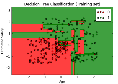

                                                                   

# Visualising the Test set results
from matplotlib.colors import ListedColormap
X_set, y_set = X_test, y_test
X1, X2 = np.meshgrid(np.arange(start = X_set[:, 0].min() - 1, stop = X_set[:, 0].max() + 1, step = 0.01),
                     np.arange(start = X_set[:, 1].min() - 1, stop = X_set[:, 1].max() + 1, step = 0.01))
plt.contourf(X1, X2, classifier.predict(np.array([X1.ravel(), X2.ravel()]).T).reshape(X1.shape),
             alpha = 0.75, cmap = ListedColormap(('red', 'green')))
plt.xlim(X1.min(), X1.max())
plt.ylim(X2.min(), X2.max())
for i, j in enumerate(np.unique(y_set)):
    plt.scatter(X_set[y_set == j, 0], X_set[y_set == j, 1],
                c = ListedColormap(('red', 'green'))(i), label = j)
plt.title('Decision Tree Classification (Test set)')
plt.xlabel('Age')
plt.ylabel('Estimated Salary')
plt.legend()
plt.show()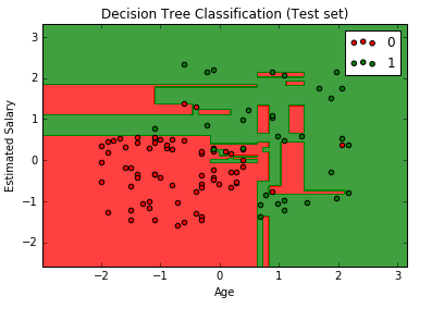

                                                            

Though the Decision Tree algorithm is good for classification of random data, it is sensitive to noisy data and has a tendency to overfit data. Even the small variance in data can result in different Decision Trees. So it is recommended to balance the dataset before fitting the algorithm to the dataset.