Learn Simple Linear Regression in the Hard Way(with Python Code) | Machine Learning

Regression models try to fit the best line to a set of observed data points. While simple linear models use a straight line, other models like multiple regression or polynomial regression use curved lines. A regressive model allows you to understand how the dependent variable changes in response to the change of independent variables.

In this tutorial, we are going to understand what is simple linear regression. We will then implement a simple linear regression model in python. So, stay tuned!

What is Simple Linear Regression?

A simple linear regression model only has two explanatory variables- one dependent and one independent variable. Think of a two-dimensional space where the horizontal axis represents the independent variable x, and the vertical axis represents the dependent variable y. Like that, a simple linear regression model uses two-dimensional sample points. The model predicts the values of the dependent variable as a function of the independent variable. It tries to find a simple linear function that represents the relationship between the independent and the dependent variable as accurately as possible. The function simply creates a straight line, more specifically a slope that resembles the prediction line. 

For example, there is a relationship between cigarette consumption and cancer. More consumption of cigarettes creates a high chance of cancer. The relationship here seems linear and the variables can be fitted in a two-dimensional space. So, we can describe this phenomenon using a simple linear regression model.

The Formula for Simple Linear Regression Model

The formula representing a simple linear regression is-

y = b0 + b1X + e

Let's interpret the equation

• y represents the predicted value of the dependent variable according to the given value of the independent variable.
• b0 represents the intercept, the value of the function when the independent variable is 0
• b1 is the regression coefficient, it tells how much the values of the function will scale to the independent variable
• X represents the independent variable of the function 
• e represents error the model is creating

With this function, a simple linear regression model will predict the dependent variable(denoted y) values as a function of the independent variables(denoted x). Basically, this function generates a straight line in the cartesian coordinate system. This straight line is the prediction line for the simple linear regression model which tries to predict the dependent values as accurately as possible.

Assumptions of Simple Linear Regression

Simple linear regression model uses a parametric test. The parametric test depends on the distribution of the data(often normal distribution). So it makes some certain assumptions about the data. There are four assumptions associated with a simple linear regression model- 

• Linearity It assumes that the relation between the data points is linear i.e. the plot of the data points shows is linear
• Independence There must be no relationship among the different values of the independent variable i.e. the value is unique
• Normality Data points follow a normal distribution i.e. if we plot the histogram of the data, we should be able to draw a skewed line
• Equal Variance The variance of the data should be equally distributed i.e. they do not "fan-out" in a triangular fashion

When your data does not meet any of the above assumptions you can not perform a simple linear regression. Rather you should use a nonparametric test.

Think about stock price data. Here observations for the same entity(stock) are collected over time. This data violates the assumption of independence and the data is also not linear. So, we can not perform linear regression on this data.

Simple Linear Regression in Python

There is a simple and easy way to build a simple linear regression model. In this tutorial, we will use the Scikit-learn module to perform simple linear regression on a data set.

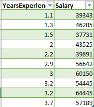
We take a salary dataset. It has two variables- years of experience and salary. Therefore, the data set is two-dimensional. Taking the experience as the independent variable and the salary as the dependent variable, let's perform a simple linear model to it.

You can download the dataset from here.

Let's plot the data in a graph.

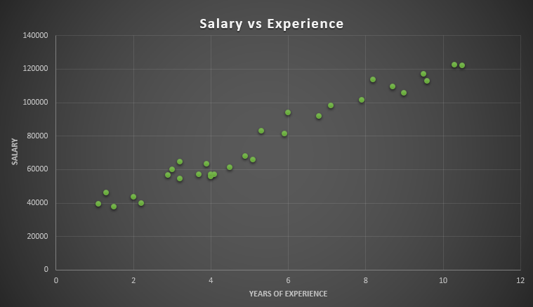
Look at the plot. The data is linear, independent, and equally distributed. So, it meets the assumptions of simple linear regression.

Now let's build a simple linear regression model with this dataset. You will get the full code in Google Colab. 

The first step will be preprocessing the dataset. As this model deals with just two variables, we can take the Experience column as the independent variable in the feature matrix X, and the Salary column as a dependent variable in the dependent variable vector y.

#Simple Linear Regression
# Importing the essential libraries
import numpy as np 
import matplotlib.pyplot as plt 
import pandas as pd 
# Importing the dataset 
dataset = pd.read_csv('Salary_Data.csv') 
X = dataset.iloc[:, 0:1].values
y = dataset.iloc[:, 1].values

Now, we will split the dataset between training and test sets. The training set will contain two-third of the data and the test set will have one-third of the data. You can try taking the arbitrary size for training and test sets. But keep in mind that the size of your datasets will make the model predict different outcomes. So, try to split the dataset in a way that helps the model to predict the best outcome.

# Splitting the dataset into the Training set and Test set 
from sklearn.model_selection import train_test_split 
X_train, X_test, y_train, y_test = train_test_split(X, y, test_size = 1/3, random_state = 0)

Note: Here, random_state = 0 is used to ensure that when you run this code, the output will be the same as us. You could run your code perfectly without this parameter. Though the training data set and test data set may not look exactly like ours, still it will be fine.

After preprocessing the data, now we will build our simple linear regression model. To fit the model to our training set, we just need to use the linear regression class from the Scikit-Learn module. The code in Python is as follows:

# Fitting Simple Linear Regression to the Training set 
from sklearn.linear_model import LinearRegression 
regressor = LinearRegression() 
regressor.fit(X_train, y_train)

Now we have come to the final part. Our model is ready and we can predict the outcome! The code for this is as follows:

# Predicting the Test set results 
y_pred = regressor.predict(X_test)

Visualize Simple Linear Regression in Python

We have come to the fun part. Now we will visualize the results in python. There are two different results. We will plot both in python.

To visualize the training set results:

# Visualising the Training set results 
plt.scatter(X_train, y_train, color = 'red') 
plt.plot(X_train, regressor.predict(X_train), color = 'blue') 
plt.title('Salary vs Experience (Training set)') 
plt.xlabel('Years of Experience') 
plt.ylabel('Salary') 
plt.show()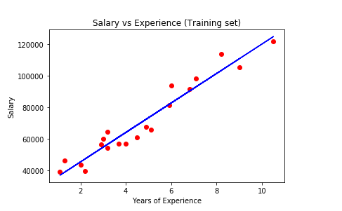

Here the graph represents the linear regression line(the blue straight line) for the training set data. The algorithm tries to find the best fit line for our dataset. So this line is the best fit line the algorithm could find for our data.

Now it is time to see how our model predicts on the test data:

# Visualising the Test set results 
plt.scatter(X_test, y_test, color = 'red') 
plt.plot(X_train, regressor.predict(X_train), color = 'blue') 
plt.title('Salary vs Experience (Test set)') 
plt.xlabel('Years of Experience') 
plt.ylabel('Salary') 
plt.show()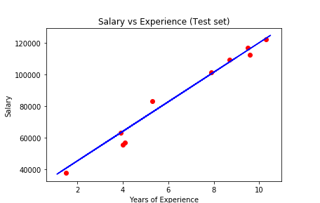

The above graph shows the predictions made by our simple linear regression model. The red dots are the test data and the blue line represents the predictions made by our model. If you look at the graph, our model made some close predictions for our test data(the dots on the line). Though the prediction is not accurate for some values(the dots far from the line), still it is a good simple linear regression model.

This is the simplest of all the regression models. In the following articles, we will see other complex regression models.

How to Improve a Simple Linear Regression Model?

The performance of our model is not that good. The regression line could not fit all the data points well. Therefore, we need improvements. There are many ways we can increase the accuracy of a simple linear regression model. Try the followings-

• Normalize the Data The data should be made normalized to get a more perfect model. There are normalizer functions you can apply to do so.
• Remove Outliers If the dataset contains outliers i.e. values outside the normal distribution, the accuracy will not be improved. Remove the outliers to get better accuracy.
• Check Collinearity If the data is correlated somehow, as I said earlier, the linear regression model will not perform well. Try to check and remove collinearity and then apply the model.

Final Thoughts

In this article, I tried to explain everything you need to learn about linear regression. Started with what linear regression is and then show you the way how it works. Finally, we implemented a linear regression model in Python. Simple linear regression is the simplest implementation of regression models. It does not perform well for many types of data i.e. data with more than two variables. So, you can not always use it. Instead, you need to use other regression models. Hope this article helped you to understand simple linear regression well. 

Happy Machine Learning!