Thompson Sampling Intuition | Machine Learning

In this article, we will talk about the Thompson Sampling Algorithm for solving the multi-armed bandit problem and implement the algorithm in Python.

Thompson Sampling Algorithm:
Thompson Sampling is one of the oldest heuristics to solve the Multi-Armed Bandit problem. This is a probabilistic algorithm based on Bayesian ideas. It is called sampling because it picks random samples from a probability distribution for each arm. This could be defined as a Beta Bernoulli sampler. Though Thompson sampling can be generalized to sample from any arbitrary distributions. But the Beta Bernoulli version of Thompson sampling is more intuitive and is actually the best option for many problems in practice. In this tutorial, we will use the Beta Benouli sampler.

Algorithm Comparison: Upper Confidence Bound vs. Thompson Sampling:
There is a significant difference between UCB and Thompson sampling. Firstly UCB is a deterministic algorithm whereas Thompson sampling is a probabilistic algorithm. In UCB you must incorporate the value at every round, you cannot proceed to the next round without adjusting the value. In Thompson, you can accommodate delayed feedback. This means you can update the dataset for your multi-armed bandit problem in a batch manner, that will save your additional computing resource or cost of updating the dataset each time. This is the main advantage of Thompson sampling over UCB.

Recently, it has generated significant interest after several studies demonstrated it to have better empirical performance compared to the UCB algorithm.

How this Algorithm Works?

Let's say we have three multi-armed bandits with the following distributions

                                       
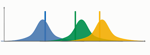
In the above distribution, our expected value can anywhere in the distribution. Now, this algorithm will choose samples from the above distribution using Bayesian Inference rules. First, it will run some trial rounds before doing the actual computation.

                                       

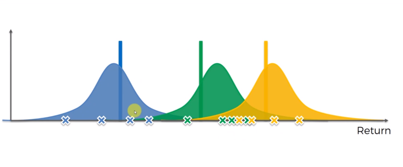
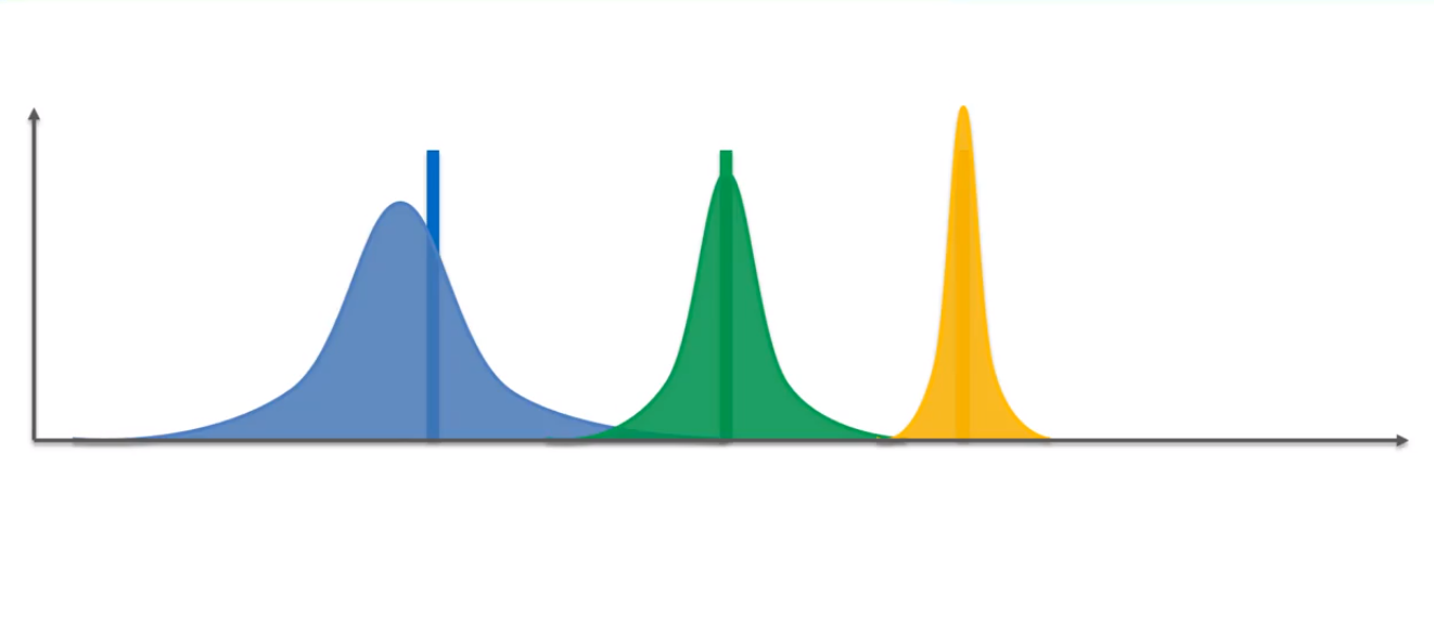
Now, it will pick the samples from each of the distributions that have the highest value of the distribution. This will make an imaginary set of bandits. That means that this algorithm actually makes an auxiliary mechanism to solve the problem, that is, it will not create the machines at every round rather it will create the possible ways these machines could be recreated. With each trial, each takes a sample that has the highest distribution. And with each trial, the distribution will be changed. The distribution will get narrower as we have some information. After a huge number of rounds, we will get the narrowest distribution which we will take as the final outcome.

                                       

Now let's look at the steps of the algorithm.

 

Let's implement this algorithm for our own version of a multi-armed bandit problem. Here we will take a dataset of online advertising campaigns where an ad has 10 different versions. Now our task is to find the best ad using the Thompson sampling algorithm.

 

Let's look at the steps we need in Thompson sampling:

              

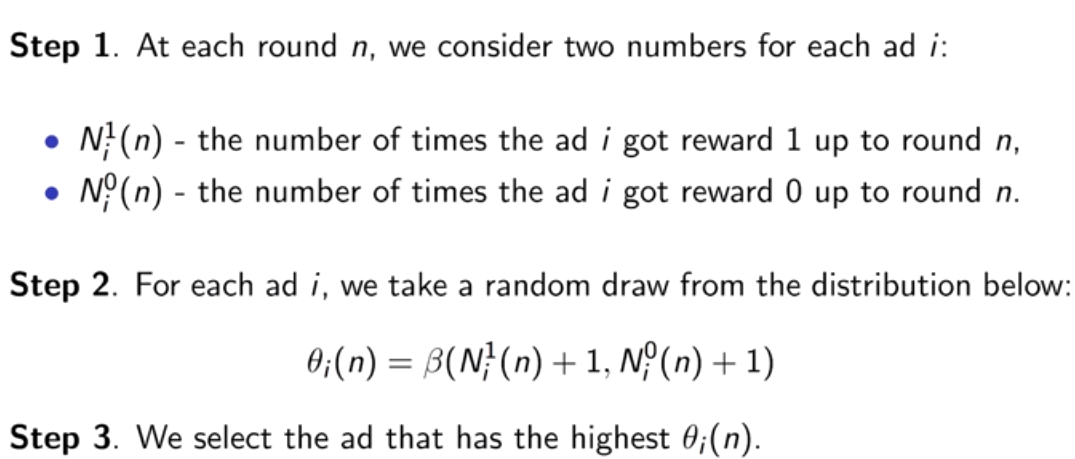
At the first step, the total number of rewards(either 0 or 1) is counted.

To understand the second step, we need to look at the Bayesian inference rules-

              
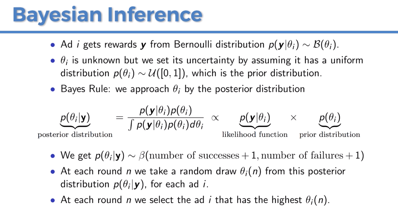
For step 2, we have two assumptions, first, we say that each ad i gets a reward from a Bernoulli distribution which is the probability of success. You can picture this parameter by showing this ad to a million users and the parameter will be interpreted as the number of times the outcomes were ones divided by the number of ads. Basically, it is the probability of getting ones. The second assumption is that we have a uniform distribution which is a prior distribution, then we have the posterior distribution from the Bayes rule that is the probability of success given the rewards after the round n. By doing this Bayes rule we get the beta distribution here. In Thompson sampling, these random draws mean nothing but the probability of success, because the maximum of these random draws approximating the highest probability of success. And this is the idea behind Thompson sampling. By taking the highest of these draws we are maximizing the probability of success for each of the 10 ads. And this highest probability corresponds to each ad at every round.  After performing the algorithm we will take the highest ad having the highest probability of success.

Thompson sampling in Python:
First of all, we need to import essential libraries. You will get the code in Google Colab also.

import numpy as np
import matplotlib.pyplot as plt
import pandas as pd

Then we will import our dataset (Ads_CTR_Optimisation.csv)

You can download the dataset from here.

# Importing the dataset 
dataset = pd.read_csv('Ads_CTR_Optimisation.csv')

Now, let's implement the Thompson Sampling code

# Implementing Thompson Sampling
import random
N = 10000
d = 10
ads_selected = []
numbers_of_rewards_1 = [0] * d
numbers_of_rewards_0 = [0] * d
total_reward = 0
for n in range(0, N):
    ad = 0
    max_random = 0
    for i in range(0, d):
        random_beta = random.betavariate(numbers_of_rewards_1[i] + 1, numbers_of_rewards_0[i] + 1)
        if random_beta > max_random:
            max_random = random_beta
            ad = i
    ads_selected.append(ad)
    reward = dataset.values[n, ad]
    if reward == 1:
        numbers_of_rewards_1[ad] = numbers_of_rewards_1[ad] + 1
    else:
        numbers_of_rewards_0[ad] = numbers_of_rewards_0[ad] + 1
    total_reward = total_reward + reward

Now, we have come to the final part of our program. Let's visualize what we got-

plt.hist(ads_selected)
plt.title('Histogram of ads selections')
plt.xlabel('Ads')
plt.ylabel('Number of times each ad was selected')
plt.show()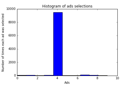

                                    

In the above histogram, you can see that ad version five has the highest probability of success. So we will take the fifth version of the ad as output. If you compare this result with our previous Upper Confidence Bound result, you will see a clear difference. Though the UCB algorithm found the same ad version as of Thompson sampling, the Thompson sampling showed better empirical evidence than UCB in practice.