Support Vector Machine(SVM) Made Easy with Python | Machine Learning

Support Vector Machine is one of the popular machine learning algorithms. I assume you have already learned the other classification algorithms like logistic regression and Naive Bayes. If you have not learned them I want you to check them before diving into SVM. Why? Because having a good knowledge of other simple classification algorithms will help you understand SVM better.

In this tutorial, we will learn the Support Vector Machine algorithm in detail. Then we will implement a Support Vector Machine in Python.

What is Support Vector Machine?

Support Vector Machine is a supervised machine learning algorithm. It can be used in both classification and regression problems. Inherently, it is a discriminative classifier. Given a set of labeled data points, an SVM tries to separate the data points into different output classes. It does so by finding an optimal hyperplane that distinctly classifies the data points into an N-dimensional space(N - the number of features). 

Before getting to the working principle of SVM, first, we need to understand some key definitions.

What is a Hyperplane in SVM?

A hyperplane is defined as an n-1 dimensional Euclidean space that separates an n-dimensional Euclidean space into two disconnected parts or classes. The "optimal" hyperplane is one that maximizes the margin between the two classes, which means the distance of the hyperplane is equal from both the nearest data points of these two classes.

In a two dimensional space, a hyperplane is a line that optimally divides the data points into two different classes. In three dimensions, a hyperplane is a 2D plane. In other higher dimensions, the hyperplane would take more complex shapes.

What is a Support Vector in SVM?

Support vectors are those two data points supporting the decision boundary(the data points which have the maximum margin from the hyperplane). An SVM always try to those two data points from different classes that are the closest to each other. These support vectors are the keys to draw an optimal hyperplane by SVM.  In SVM, the set of input and output data are treated as vectors. This is because when the data is a higher-dimensional space(more than two dimensions), the classes cannot be represented as single data points, so they must be represented as vectors. And that's how it's got the name "Support Vector Machine".

How Does Support Vector Machine Work?

In the above, we got an intuitive idea of SVM. Now, we will see how the algorithm actually separates the classes. There can be two scenarios for an SVM depending on the nature of data. Data can be of two types- linearly separable or non-linearly separable. Let's understand the working procedure of SVM for both cases.

Scenario 1: Data is linearly separable

To see what data is linearly separable, consider the following data plot-

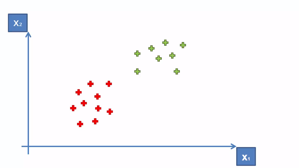
Here the data is linearly separable because you can separate them into two classes just with a line. This line is known as the hyperplane in sense of and SVM. As we discussed earlier, SVM will find an optimal hyperplane that will separate the data into two "distinct" classes. This line can be drawn anywhere on the plane-

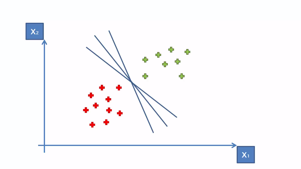
In the above, any of the lines can separate the classes. But we need to take the optimal one, right? Here where the Support vectors come into play. SVM will find those two boundary data points or support vectors. These support vectors should be at a maximum margin from the optimal hyperplane. 

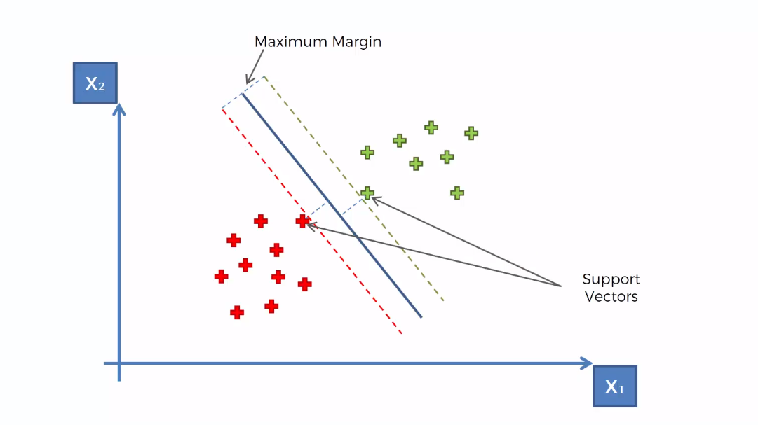
This illustration tells us everything. You see the SVM finds the two closest support vectors and separates the classes with the optimal hyperplane.

Scenerio 2: Data is not linearly separable

What if our data is in a more complex shape that they can not be linearly separable? Look at the following illustration-

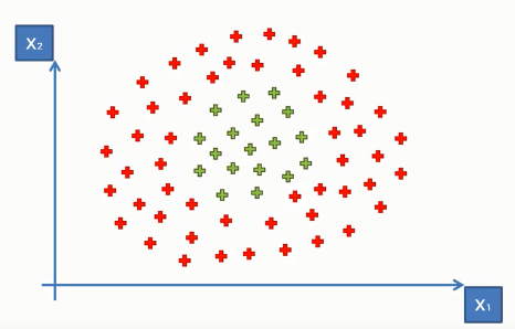
You see clearly there are two classes. But we can not separate them(you may try splitting with a knife!). Jokes apart, we can not separate them as the data is not linearly separable. But SVM can. What it does in this sense that it takes the data into a higher dimension. In a higher dimension, the data will be in different shapes and hence can be linearly separable.

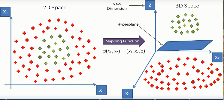
You can see, taking the data into three-dimensional space, they become linearly separable by a 2D hyperplane. SVM creates a mapping function that elevates the data into a higher dimension. There it tries to find the optimal hyperplane. Recall how SVM finds it in the previous example. Then it projects back the data into its original dimension. Now, the data is well separated into two distinctive classes.

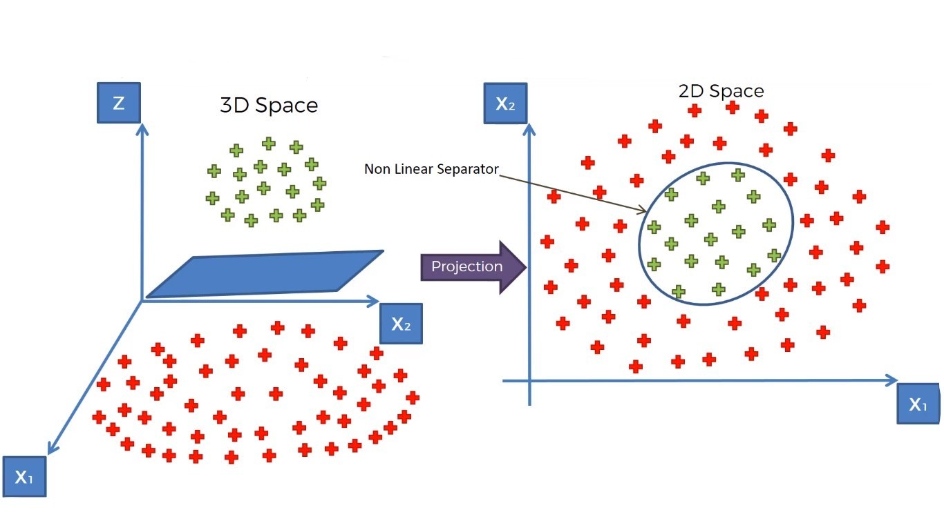
This is the whole idea of working with non-linear data. These mapping functions are made of special mathematical functions called the kernel trick.

SVM Kernel Explained

As we have seen, we can separate non-linearly separable data by taking them into a higher dimension. In our example, we need to map the data into just one dimension higher. But in most cases, we need to take higher dimensions to make the data linearly separable. Now, think about how much the computation cost would be to take the data into higher dimensions and remap them into the original dimensional? The operation will be costly.

This is where the kernel trick comes into play. It allows us to calculate the data into a higher-dimensional space still remaining in our original feature space. In simple terms, Kernel Tricks are functions that apply some complex mathematical operations on the lower-dimensional data points and convert them into higher dimensional space.  Then finds out the process of separating the data points based on the labels and outputs we have defined. This is less expensive and fast.

Different Types of Kernels in SVM

There are many types of kernels are used in SVM. Some of the common kernels are-

• Linear Kernel
• Polynomial Kernel 
• Radial Basis Function of RBF Kernel
• Sigmoid Kernel
• Gaussian Kernel

Which Kernel is Best for SVM?

There is no rule of thumb for a standard kernel in SVM. The choice of a kernel is data specific. Sometimes linear kernel works well for the data. If not, then you might go with Polynomial or Gaussian kernels. Though we can not say how good a kernel will be before using a kernel, in practice, the Gaussian kernel is the most widely used kernel. It works extremely well for well-behaved data i.e. data with no or less noise. For special-purpose problems or domains, you need to use more customized kernels. For instance, a graph kernel might be good when you want to classify graphs in a network or a string kernel is a good option for working with genetic data.

Support Vector Machine in Python

Now we will implement this algorithm in Python. For this task, we will use the dataset Social_Network_Ads.csv. Let's have a glimpse of that dataset.

                                                      

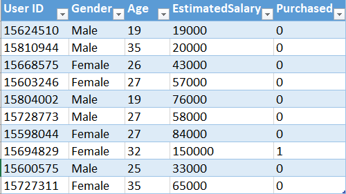
This dataset contains the buying decision of a customer based on gender, age and salary. Now, using SVM, we need to classify this dataset to predict the decision for unknown data points.

You can download the whole dataset from here.

First of all, we need to import the essential libraries to our program. You will get the code in Google Colab also.

import numpy as np
import matplotlib.pyplot as plt
import pandas as pd

Now, lets import the datset.

dataset = pd.read_csv('Social_Network_Ads.csv')

In the dataset, the Age and EstimatedSalary columns are independent and the Purchased column is dependent. So we will take both the Age and EstimatedSalary in our feature matrix and the Purchased column in the dependent variable vector.

X = dataset.iloc[:, [2, 3]].values
y = dataset.iloc[:, 4].values

Now, we will split our dataset in training and test sets.

from sklearn.model_selection import train_test_split
X_train, X_test, y_train, y_test = train_test_split(X, y, test_size = 0.25, random_state = 0)

We need to scale our dataset for getting a more accurate prediction.

from sklearn.preprocessing import StandardScaler
sc = StandardScaler()
X_train = sc.fit_transform(X_train)
X_test = sc.transform(X_test)

Well, its time to fit the SVM algorithm to our training set. For this, we use the SVC class from the ScikiLearn library.

from sklearn.svm import SVC
classifier = SVC(kernel = 'linear', random_state = 0)
classifier.fit(X_train, y_train)

Note: Here kernel specifies the type of algorithm we are using. You will know about it in detail in our Kernel SVM tutorial. For simplicity, here we choose the linear kernel.

Our model is ready. Now, let's see how it predicts for our test set.

y_pred = classifier.predict(X_test)

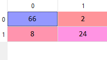
To see how good is our SVM model is, let's calculate the predictions made by it using the confusion matrix.

from sklearn.metrics import confusion_matrix
cm = confusion_matrix(y_test, y_pred) 

The output of the confusion matrix will be

                                   

Visualizing Support Vector Machine in Python

Now, let's visualize our test set result.

# Visualising the Test set results
from matplotlib.colors import ListedColormap
X_set, y_set = X_test, y_test
X1, X2 = np.meshgrid(np.arange(start = X_set[:, 0].min() - 1, stop = X_set[:, 0].max() + 1, step = 0.01),
                     np.arange(start = X_set[:, 1].min() - 1, stop = X_set[:, 1].max() + 1, step = 0.01))
plt.contourf(X1, X2, classifier.predict(np.array([X1.ravel(), X2.ravel()]).T).reshape(X1.shape),
             alpha = 0.75, cmap = ListedColormap(('red', 'green')))
plt.xlim(X1.min(), X1.max())
plt.ylim(X2.min(), X2.max())
for i, j in enumerate(np.unique(y_set)):
    plt.scatter(X_set[y_set == j, 0], X_set[y_set == j, 1],
                c = ListedColormap(('red', 'green'))(i), label = j)
plt.title('SVM (Test set)')
plt.xlabel('Age')
plt.ylabel('Estimated Salary')
plt.legend()
plt.show()

The graph will like the following

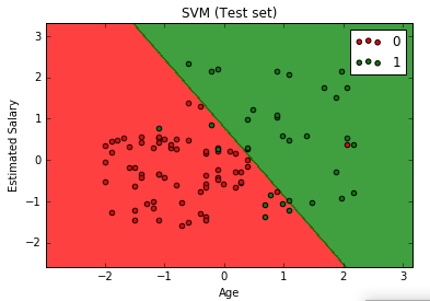
From the above graph, we can see that our model tries to find the optimal line that separates the data points accurately.

This tutorial only explains SVM in two-dimensional space, in the next tutorial we will see SVM in higher dimensional spaces.

Multiclass SVM Explanation

Support Vector Machines are inherently binary classifiers. This is why it is called one of classifier. But in many cases, especially in text classification, one of classification problems are rare. For example, take some text data like China, Coffe, UK, where they can be relevant to many topics. However,  to perform multiclass classification with SVM, we can apply one of the following strategies-

• Build a one-versus-rest classifier or commonly known as the One-Versus-All(OVA) classifier. Then choose the class which classifies the test data with highest margin. The training time is higher in this case as you have to take all the training data for one classifier.
• Build a set of OVA classifiers. Then choose the class that is selected by the highest number of classifiers. This approach reduces the training time since the training data is distributed to each classifier.

The two above mentioned methods are quite general and not a very elegant approach to solving multiclass problems. A better approach is to build a multiclass SVM which could naturally deal with multiclass problems.

The construction of a multiclass SVM is quite complex and beyond the scope of this tutorial. I suggest you check this implementation to learn more about the multiclass support vector machines.

What is the Difference Between SVM and LinearSVC?

LinearSVC stands for Linear Support Vector Classification. It is similar to SVC in terms of the kernel parameter(when kernel='linear'). But the difference is in implementation. SVC implemented in terms of libsvm whereas LinearSVC is implemented in terms of liblinear. It makes it more flexible in the choice of penalties and loss functions. This class supports both dense and sparse inputs. The multiclass classification is handled by using one-vs-all(OVM) strategy.

Talking about performance, LinearSVC can perform better than SVC when there is a large number of data.

Advantages and Disadvantages of Support Vector Machine

There are some key benefits to choose a support vector machine for classification. There are some drawbacks as well. Let's talk about them-

The key advantages are-

• SVM works really well with high dimensional data. If your data is in higher dimensions, it is wise to use SVM.
• For data with a clear margin of separations, SVM works relatively well.
• When data has more features than the number of observations, SVM is one of the best algorithms to use.
• As a discriminative model, it need not memorize anything about data. Therefore, it is memory efficient. 

Some drawbacks are-

• It is a bad option when the data has no clear margin of separation i.e. the target class contains overlapping data points.
• It does not work well with large data sets.
• For being a discriminative model, it separates the data points below and above a hyperplane. So, you will not get any probabilistic explanation of the output.
• It is hard to understand and interpret SVM as its underlying structure is quite complex.

Final Thoughts

The tutorial is designed in a way to provide all the essential concepts you need to learn about Support Vector Machine. We have learned what SVM is and how it works. We understood different angles of SVM for linear and non-linear data. Then we implemented it in python. We also tried to understand the multiclass classification with SVM. We further discussed the advantages and disadvantages of SVM. 

This article is a simple yet intuitive explanation of SVM. You should read more mathematical theories behind SVM to get a deep understanding of this powerful algorithm. Hope this article could help you make this thing clearer. What do you think? Let me know in the comments.

Happy Machine Learning!