Naive Bayes Classification Just in 3 Steps(with Python Code) | Machine Learning

Naive Bayes provides a probabilistic approach to solve classification problems. Extending the Bayes Theorem, this algorithm is one of the popular machine learning algorithms for classification tasks. It provides a quantitative approach to understand the effect of observing data on each target class. 

For many learning tasks such as text mining or document classification, Naive Bayes gives the optimal result than most other classification algorithms. This effectiveness will be discussed in later parts of this tutorial. 

In this tutorial, we are going to learn the intuition behind the Naive Bayes classification algorithm and implement it in Python. So, let's dive into it!

What is Bayes Theorem?

In various machine learning tasks, we often need to determine the best hypothesis(here, a hypothesis can be seen a question about an event i.e. will it rain if the weather seems windy or not). We want the probability of a hypothesis to make a decision on it. For example, which is highly probable: it rains when the weather windy or not. After knowing the probability of these two different hypotheses, we will choose one that has the highest probability. Here we will present some prior probabilities against our hypothesis i.e. the probabilities of raining in windy weather.

Bayes theorem provides a way to calculate such probabilities. It considers various prior probabilities of hypothesis and observed data. Then it calculates the posterior probability of a hypothesis against the observing data. This posterior probability will then be the ground of our decision making.

In simple words, for a hypothesis H and observed data D and given the prior probabilities of the hypothesis, it simply calculates the maximum posterior probability of the hypothesis after observing the data.

Mathematically, 

             

Here,

• P (H | D) = Posterior probability of a hypothesis. The conditional probability for hypothesis H to occur after the data D has been observed. 
• P (H) and P (D) = The probability of  H and D to occur independently. It is assumed that P(H) and P(D) had no correlation before the observation. 
• P (D | H) = The probability of observing data D in the presence of the hypothesis H. It is also known as the likelihood of the event.

How Naive Bayes Classifier Works?

Naive Bayes classifier uses the assumption of Bayes theorem to identify the maximum probabilities of a target class. The target classes can be thought of as the hypotheses. The classifier calculates the posterior probability of each target class and outputs the class with the maximum posterior probability.

Why Do We Call It Naive?

Naive Bayes classifier makes two fundamental assumptions on the observations-

• The target classes are independent of each other. Think of a rainy day when the weather is both windy and humid. A Naive classifier would take these two features, wind and humidity as independent of each other. That means each feature would impose its own probabilities on the result, here rain.
• The target classes have an equal prior probability. That means before calculating the posterior probability of each class, the classifier will give the same prior probability to each target class.

For these assumptions, a naive Bayes could implement a more generalized form of a Bayes theorem. This is why we call it "Naive" or "Idiot".

Let's take an example. We have a dataset where the age and salary of people are taken and upon these features, the choice of an individual whether he/she will go office walking or driving is observed.

We have 30 observations available fo those distinctive features. In the below illustration, the red ones represent people walking to the office and green ones for people driving to the office.

                                

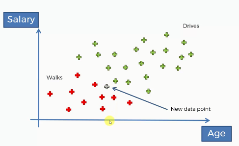
Now, for a new observation(the grey data point), we need to classify which class does it belong to. That means we should find whether this new person walks or drive. For this, we will apply the Naive Bayes technique to take the decision.

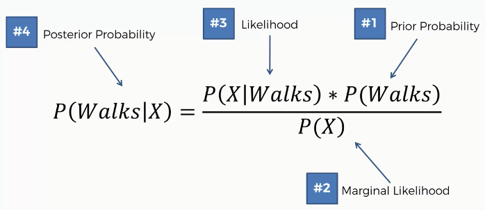
First of all, we will apply Bayes Theorem to calculate the posterior probability of walking for this new data point based on the given features X. That is how likely the person walks.

                                           

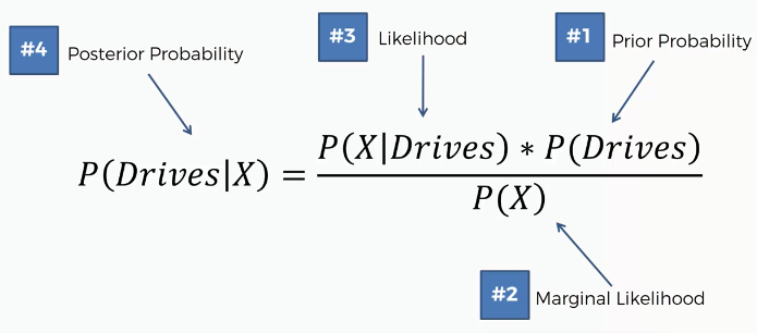
In the same way, we will calculate the probability of driving

                                            

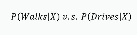
After calculating both the probabilities, the algorithm will compare them, and take the one that has the highest value.

                                            

Let's apply the Naive Bayes Algorithm in three steps-

Step 1: Now we will calculate all the prior probability, marginal likelihood, likelihood, and posterior probability of a person likely to walk.

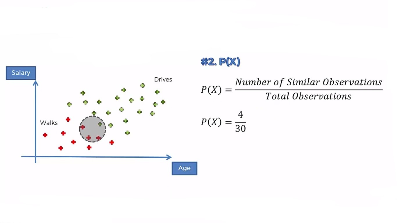
The prior probability, P(Walks) is simply the probability of the persons who walk among all the people. 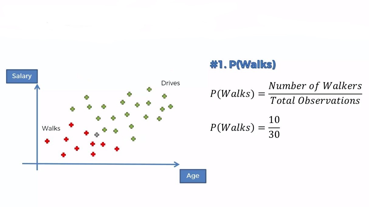                                    For marginal likelihood, P(X), we will make a circle around the new data point and calculate all the observations (including red and green). The radius of the circle depends upon you. That means you can take different radii depending on the algorithm.             

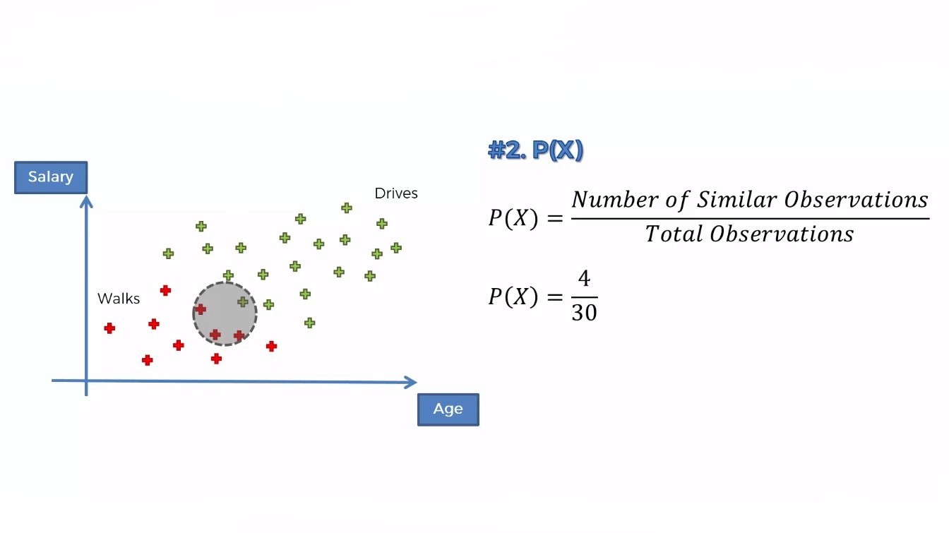
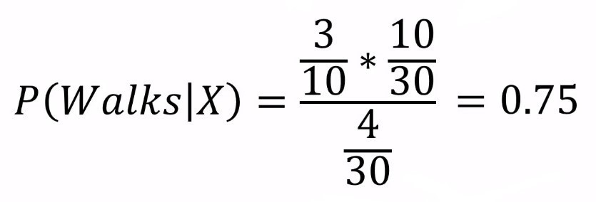
The likelihood is the probability of such persons who walk to work. So, here we are concerned only with the red dots.                           

After calculating all these, now we can put them into the Bayes' Theorem

                             

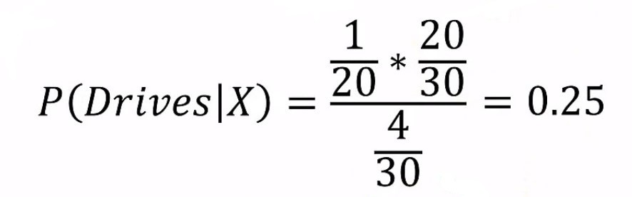
Step 2: Now, we will do similar calculations for P(Drives | X)

                   

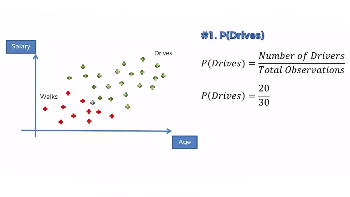
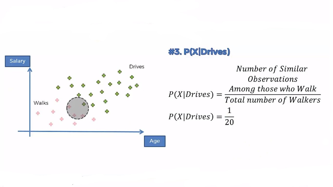
Putting all these together, we get-

                       

                      

   

Step 3: Now we will compare both the probabilities. Then we will take the higher probability value as the output.

                           

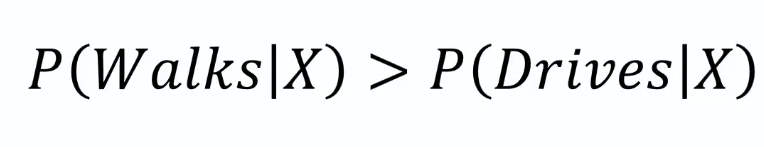
Here we can see the probability of a person likely to walk is greater than the probability for a person to drive. So we say that our new point falls into the category of people who walks.

Naive Bayes Classifier in Python

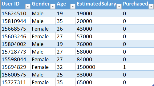
Now, we will implement the algorithm in Python. For this task, we will use the Social_Network_Ads.csv dataset. Let's have a glimpse of that dataset-

                                                    

Problem Statement

A company has provided the above dataset they collected while advertising for a specific product on social media. The dataset contains three attributes-Gender, Age, and Estimated Salary of people surveyed by a company. The target class is Purchased where based on the other three attributes the buying decision of a person is observed. The output has two classes-0 and 1. 0 means the customer did not buy the product, 1 means they buy one. So, this is clearly, a classification problem. The company wants us to build a machine learning model that will be trained upon the data. They will use the model to determine the most potential customers to advertise and maximize their profit.

Now, our task is to use this dataset to train a classifier with the data to build a predictive model. We will use Naive Bayes Classifier for that purpose

You can download the whole dataset from here.

First of all, we will import all the essential libraries. You will get the code in Google Colab also.

# Importing essential libraries 
import numpy as np 
import matplotlib.pyplot as plt 
import pandas as pd

Now, we will import the dataset to our program

# Importing the dataset 
dataset = pd.read_csv('Social_Network_Ads.csv')

From the dataset, we take the Age and EstimatedSalary columns in the Feature matrix as they are independent features and the Purchased column in the Dependent vector. 

# Making the Feature matris and dependent vector 
X = dataset.iloc[:, [2, 3]].values 
y = dataset.iloc[:, 4].values

Now, we split our dataset into training and test sets.

# Splitting the dataset into the Training set and Test set 
from sklearn.model_selection import train_test_split 
X_train, X_test, y_train, y_test = train_test_split(X, y, test_size = 0.25, random_state = 0)

We need to scale the training and test sets to get a better prediction.

#Feature Scaling 
from sklearn.preprocessing import StandardScaler 
sc = StandardScaler() 
X_train = sc.fit_transform(X_train) 
X_test = sc.transform(X_test)

Now, we will fit the Naive Bayes algorithm to our dataset. 

# Fitting Naive Bayes to the Training set 
from sklearn.naive_bayes import GaussianNB 
classifier = GaussianNB() 
classifier.fit(X_train, y_train)

Its time to see how our model predicts the test set result.

# Predicting the Test set results 
y_pred = classifier.predict(X_test)

We will see the performance of our model using the confusion matrix.

# Making the Confusion Matrix
from sklearn.metrics import confusion_matrix
cm = confusion_matrix(y_test, y_pred)

Now, we will visualize our model with the training set result.

# Visualising the Training set results 
from matplotlib.colors import ListedColormap 
X_set, y_set = X_train, y_train 
X1, X2 = np.meshgrid(np.arange(start = X_set[:, 0].min() - 1, stop = X_set[:, 0].max() + 1, step = 0.01), np.arange(start = X_set[:, 1].min() - 1, stop = X_set[:, 1].max() + 1, step = 0.01))
plt.contourf(X1, X2, classifier.predict(np.array([X1.ravel(), X2.ravel()]).T).reshape(X1.shape), alpha = 0.75, cmap = ListedColormap(('red', 'green'))) 
plt.xlim(X1.min(), X1.max()) 
plt.ylim(X2.min(), X2.max()) 

for i, j in enumerate(np.unique(y_set)): 
    plt.scatter(X_set[y_set == j, 0], X_set[y_set == j, 1], c = ListedColormap(('red', 'green'))(i), label = j) 

plt.title('Naive Bayes (Training set)') 
plt.xlabel('Age') 
plt.ylabel('Estimated Salary') 
plt.legend() 
plt.show()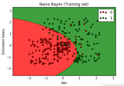

                         

We will now see how it performs on our test set. Let's visualize this.

# Visualising the Test set results 
from matplotlib.colors import ListedColormap 
X_set, y_set = X_test, y_test 
X1, X2 = np.meshgrid(np.arange(start = X_set[:, 0].min() - 1, stop = X_set[:, 0].max() + 1, step = 0.01), np.arange(start = X_set[:, 1].min() - 1, stop = X_set[:, 1].max() + 1, step = 0.01)) plt.contourf(X1, X2, classifier.predict(np.array([X1.ravel(), X2.ravel()]).T).reshape(X1.shape), alpha = 0.75, cmap = ListedColormap(('red', 'green'))) 
plt.xlim(X1.min(), X1.max()) 
plt.ylim(X2.min(), X2.max()) 
for i, j in enumerate(np.unique(y_set)): 
    plt.scatter(X_set[y_set == j, 0], X_set[y_set == j, 1], c = ListedColormap(('red', 'green'))(i), label = j) 

plt.title('Naive Bayes (Test set)') 
plt.xlabel('Age') 
plt.ylabel('Estimated Salary') 
plt.legend() 
plt.show()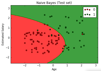

                            

Different Types of Naive Bayes Classifier

In Scikit-Learn documentation, five variants of the Naive Bayes algorithm are implemented. They are-

• Gaussian Naive Bayes For continuous features, it is widely used. It assumes that the features are in Gaussian distribution that represents a continuous bell curve.
• Multinomial Naive Bayes It is specially designed to use in-text classification where the data are generally multinomial, represented as word vector counts. For example, in document classification, It works like the following- While training, It explicitly takes into account the words counts and adjusts the underlying probabilities according to that. Unlike a simple naive Bates, which models a document as the presence or absence of some particular words.
• Complement Naive Bayes It is a special adaptation of the multinomial naive Bayes classifier which implements the complement naive Bayes(CNB) algorithm. It is particularly designed to suit imbalanced data sets. It uses statistics from the complement of each class to calculate the weight of the model. For imbalanced data sets, the parameter estimates for CNB are more stable than those for other classifiers.
• Bernoulli Naive Bayes This algorithm is implemented with data that follows multivariate Bernoulli distributions. There may be multiple features but it assumes each feature to be a binary-valued(Bernoulli or boolean) variable. For text classification purposes, word occurrence vectors instead of the word count vectors may be used to train and use this classifier. In most cases, Bernoulli Naive Bayes performs better on datasets of shorter documents. But you should evaluate both this and the multinomial Naive Bayes classifier to check which is better in a specific dataset.
• Categorical Naive Bayes It implements Naive Bayes Algorithm for categorically distributed data. It assumes each feature described by the index, has its own categorical distribution. It also assumes that the categorical values are encoded i.e. each feature is represented with numbers. When the features are mostly categorical, this classifier could be a good choice for classification.

Improving Accuracy: Ways to Build A More Efficient Naive Bayes Classifier

Naive Bayes itself a robust classifier and can perform very well in any form of data. But it can be improved for more accurate performance. Specially for text classification where Naive Bayes Classifier is more frequently used. We discover many issues when working with text classification. Here, some of the ways are discussed to get the best from your model-

Gather Enough Data

This is the first thing you should do. Though Naive Bayes does not require a huge amount of data to find the probabilities of the features. But you should provide enough data that can explain most of the distribution of the data.

Better Data Preprocessing

Text data are messy. They require a good amount of effort in the pre-processing stage to make them more useful to the classifier to learn. While preprocessing your data, must do the followings-

• Stemming Stemming will help you to reduce the size of words in the text. Suppose your texts contain love, lovely, loving, loved, lovable all having a same root word love. Stemming will reduce all the words to a single root word. This makes the vector less complicated.
• Group Synonyms This is a similar idea to stemming. It will convert words with a similar meaning into one single word. For example, lovely, fine, attractive, charming all are synonyms to beautiful. This will roll everything to a single term.
• Remove Stop Words Stop words are those words that have little or no importance to the final output. Removing them will help you create a better data set.
• Correct Spelling Mistakes Try to ensure your training data are mistakes free. This will help the classifier to learn better from the data.

Use Feature Selection Methods

If your data set contains a large number of features, this will increase the computational complexity of the classifier. So, before building the model, make sure that your data has fewer features. You can apply various feature selection methods to do so.

Remove Correlated Features

Naive Bayes assumes that the features are independent of each other. So, correlated features will affect the performance of the probability classification. You need to remove correlated features to improve accuracy.

Tune the Parameters

The accuracy can be changed for different types of data. The classifier parameters will also perform differently for different types of data. Tune your parameters to the specific types of your data.

Apply Classifier Combination

You should apply some kind of classifier combination techniques such as boosting, assembling, or bagging to your Naive Bayes classifier to make it stronger. Combinations of several classifiers will reduce the variance of the data. Though Naive Bayes does not depend on the variance, this certainly boosts accuracy. This article shows a combination of Naive Bayes and SVM(NBSVM) for better text classification accuracy.

Pros and Cons of a Naive Bayes Classifier

Using Naive Bayes you'll get many advantages over other classifiers. There are some disadvantages as well. Let's have a look at them-

Pros

• Less Training Time This algorithm only requires the entire data set once in the training time to calculate the posterior probabilities of each value of the features. That's why it is fast and takes less training time. So, for larger data sets, it is a feasible choice for most data scientists.
• Quick Prediction Since Naive Bayes pre-calculates all the probabilities, the prediction time of this algorithm is very efficient.
• Simple and Easy Since Naive Bayes is based on the posterior probabilities of each conditional feature, it is easy to understand which features are influencing the predictions. It is also easy to understand and analyze the Naive Bayes model.
• Good at Categorical Inputs When the input variables are categorical, it performs extremely well than other classification algorithms.

Cons 

• Assumption of Independence The main disadvantage with Naive Bayes is that it assumes the target classes independent of each other. But in real life, it is impossible to assure that the classes are completely independent.
• Zero Frequency Problem If it finds a category in test data that was not present in the training set, the classifier assigns a probability value of 0 to that. This will make it hard to predict. Using smoothing techniques such as Laplace Estimation, we can solve this problem.
• Bad Estimator Though it is known as a decent classifier, it has a disgrace for being a bad estimator. The reason behind the problem is that it assumes the classes are independent of each other. But in reality, there is some sort of collinearity among the features. Hence the treatment of each feature as independent makes the probability outcomes flawed. That is why in Scikit-Learn documentation, the prdict_proba outputs are not good indicators of the classifier performance. And it should not be taken seriously. 

Naive Bayes FAQs

Below I have explained some of the most common questions arise when we work with naive Bayes Classifier Why is Naive Bayes Fast?

Why is Naive Bayes Fast?

Naive Bayes is fast because all it needs in training time is the prior probabilities of the features. Which is taken once and used every time when calculating the posterior probabilities of the features. Both the prior and posterior probabilities are stored for calculating future inferences. This requires minimal use of aromatic operations like addition, multiplication. Those extremely simple computations reduce the training time and make the naive Bayes classifier amazingly fast!

Why is Naive Bayes Better than Decision Trees? 

There is no such universal classifier that performs better than other classifiers every time. Both naive Bayes and Decision trees are suitable for different types of data and you can not decide which is better without evaluating both classifiers on the same data. But in some special cases, there are some comparative advantages of naive Bayes. Such as-

• It performs better on small datasets where decision trees require more data.
• Faster in processing while decision trees take more time on training.
• Proves to be lesser overfitting data than the decision trees.

Can we Overfit a Naive Bayes Model?

Naive Bayes classifiers are extremely immune to overfishing. This is because it assumes independence among the features which may make it highly biased to some extent but gives less chance to be overstated. That does not mean naive Bayes does not overfit. But the chances are very rare to overfit the model.

How does Multicollinearity Effect the Naive Bayes Classifier?

Multicollinearity happens when two or more variables carry the same information. This condition may lead the model to be biased towards a variable. But it will not affect the Naive Bayes classifier because in Naive Bayes the features are assumed to be independent of each other. That means the presence of one feature does not affect the presence or absence of other features no matter how much the features are interrelated. So, multicollinearity does not pose any threat to a Naive Bayes classifier.

Is Gaussian Naive Bayes Linear?

In general, naive Bayes classifiers are not linear. But Gaussian naive Bayes classifier is linear because it uses exponential functions for the likelihood factors. This leads the classifier to a linear decision boundary, making it a linear classifier.

Final Thoughts

This was a lengthy tutorial indeed! We tried to cover every important aspect of the naive Bayes classifier. A quick summary of the key understanding of the above discussions is-

• What is Bayes theorem and how it works for naive Bayes classifier
• Implementation of a naive Bayes classifier in Python
• Types of naive Bayes classifier
• How to improve a naive Bayes classification model
• The pros and cons of using it

I tried to explain all the concepts as simply as possible. Hope this tutorial helped you to understand all the important topics related to naive Bayes classifier. What are your thoughts on this algorithm? Please share it with us in the comments.

Happy Machine Learning!