Multiple Linear Regression in Python (The Ultimate Guide) | Machine Learning

In this tutorial, we are going to understand the Multiple Linear Regression algorithm and implement the algorithm with Python.

Tutorial Overview

• What is Multiple Linear Regression?
• Implement Multiple Linear Regression in Python
• Improve Multiple Linear Regression model
• Implement Backward Elimination in Python

What is Multiple Linear Regression?

Multiple Linear Regression is closely related to a simple linear regression model with the difference in the number of independent variables. Whereas the simple linear regression model predicts the value of a dependent variable based on the value of a single independent variable, in Multiple Linear Regression, the value of a dependent variable is predicted based on more than one independent variable.

The Formula for Multiple Linear Regression

The concept of multiple linear regression can be understood by the following formula-

y = b0+b1*x1+b2*x2+..........+bn*xn

In the equation, y is the single dependent variable value of which depends on more than one independent variable (i.e. x1,x2,...,xn).

For example, you can predict the performance of students in an exam based on their revision time, class attendance, previous results, test anxiety, and gender. Here the dependent variable(Exam performance) can be calculated by using more than one independent variable. So, this the kind of task where you can use a Multiple Linear Regression model.

Implement Multiple Linear Regression in Python

Now, let's do it together. We have a dataset(Startups.csv) that contains the Profits earned by 50 startups and their several expenditure values. Les have a glimpse of some of the values of that dataset-

                                                 

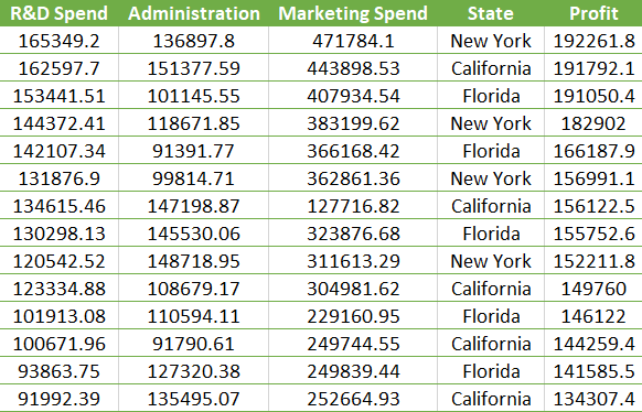
Note: this is not the whole dataset. You can download the dataset from here.

From this dataset, we are required to build a model that would predict the Profits earned by a startup and their various expenditures like R & D Spend, Administration Spend, and Marketing Spend. Clearly, we can understand that it is a multiple linear regression problem, as the independent variables are more than one.

Let's take Profit as a dependent variable and put it in the equation as y and put other attributes as the independent variables-

Profit = b0 + b1*(R & D Spend) + b2*(Administration) + b3*(Marketing Spend)

From this equation, hope you can understand the regression process a bit clearer.

Now, let's jump to build the model, first the data preprocessing step. Here we will take Profit as in the dependent variable vector y, and other independent variables in feature matrix X. You will get the full code in Google Colab.

# Importing the essential libraries
import numpy as np 
import matplotlib.pyplot as plt 
import pandas as pd 

#Importing the dataset 
dataset = pd.read_csv('50_Startups.csv') 
X = dataset.iloc[:, [0,1,2,3]].values 
y = dataset.iloc[:, 4].values

The dataset contains one categorical variable. So we need to encode or make dummy variables for that.

# Encoding categorical data
from sklearn.preprocessing import LabelEncoder, OneHotEncoder
labelencoder = LabelEncoder()
X[:, 3] = labelencoder.fit_transform(X[:, 3])
onehotencoder = OneHotEncoder()
X = onehotencoder.fit_transform(X).toarray()

Solving the Dummy Variable Trap

 The above code will make two dummy variables(as the categorical variable has two variations). And obviously, our linear equation will use both dummy variables. But this will make a problem. Here both dummy variables are correlated to some extent(that means one's value can be predicted by the other)  which causes multicollinearity, a phenomenon where an independent variable can be predicted from one or more than one independent variable. When multicollinearity exists, the model cannot distinguish the variables properly, therefore predicts improper outcomes. This problem is identified as the Dummy Variable Trap.

To solve this problem, you should always take all dummy variables except one from the dummy variable set.

#Avoiding the Dummy Variable Trap 
X = X[:, 1:]

Now split the dataset into a training set and test set

#Splitting the dataset into the Training set and Test set
from sklearn.model_selection import train_test_split
X_train, X_test, y_train, y_test = train_test_split(X, y, train_size = 0.8, test_size = 0.2, random_state = 0)

Its time to fit Multiple Linear Regression to the training set.

# Fitting Multiple Linear Regression to the Training set 
from sklearn.linear_model import LinearRegression 
regressor = LinearRegression() 
regressor.fit(X_train, y_train)

Let's evaluate our model how it predicts the outcome according to the test data. 

#Predicting the Test set result 
y_pred = regressor.predict(X_test)

Now, check how our model performed. For this, we will use the Mean Squared Error(MSE) metric from the Sciki-Learn library.

from sklearn.metrics import mean_squared_error 
print("The Mean Squared Error is- {}".format(mean_squared_error(y_test, y_pred))) 

The Mean Squared Error is- 83502864.03257468

The mean absolute error says our model has performed really bad on the test set. But we can improve the quality of the prediction by building a Multiple Linear Regression model with methods such as Backward Elimination, Forward Selection, etc. which we are going to discuss in the next chapter.

Improve Multiple Linear Regression Model

There are several ways to build a multiple linear regression model. They are-

• All In In this method, all the independent variables are included in the model. The above model is built using this method. This is the simplest one but has serious drawbacks such as allowing colinear or redundant features in the model. In most cases, the model produces bad predictions.
• Backward Elimination It is a feature selection technique where all the insignificant features are eliminated. The final model will be built using the most important features or independent variables that have the most impact on the outcome.
• Forward Selection Opposite to the backward elimination method, this method starts with an empty model and adds independent variables one by one. In every forward step, the method adds the one variable which has the most impact on the outcome.
• Bidirectional Elimination This is a combination of the above two methods. In each step, the method checks if variables can be included or excluded to improve the outcome.

In the tutorial, We are going to apply the backward elimination technique to improve our model. The steps involved in this technique are as follows-

Step 1: Select a statistical parameter e.g. p-value and set a significance level( e.g. p=0.05). A feature will be eliminated if it crosses this significance level.

Step 2: Fit the model with all the predictors

Step 3: Check the predictor with the highest p-value, if p>0.05 go to step 4. If there is no such variable, your model is ready

Step 4: Remove the predictor

Step 5: Fit the model without this predictor. 

Step 6: Repeat the 3rd, 4th, and 5th steps until you remove all the predictors above the significance level.

Implementing Backward Elimination in Python

Now, we will implement the backward elimination with our dataset to get an improved model than the previous one. For this task, we need to use the statsmodels api.

In our independent variable matrix, there is no column for constants. First of all, we need to append a constant column filled with 1's to the original matrix. Then we will make a list of all the features to build the initial model.

import statsmodels.formula.api as sm 
X = np.append(arr=np.ones((50,1)).astype(int), values=X, axis=1) 
X_pred = X[:, [0, 1, 2, 3, 4, 5]]

In the second step, we will fit the list of predictors with a regressor model.

Ols_regressor = sm.OLS(endog=y, exog=X_pred).fit()

Let's check statistics

Ols_regressor.summary()

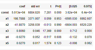
If you look at the p-value column, you can see, the third variable(Administration spend) has the highest p-value. So, in the next step, we are going to remove it and fit the model again with the rest variables.

X_pred = X[:, [0, 1, 2, 4, 5]] 
Ols_regressor = sm.OLS(endog=y, exog=X_pred).fit() 
Ols_regressor.summary()

Again check the p-value

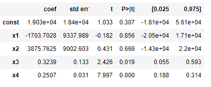
The 3 rd variable(marketing spend) has a higher p-value than the significance level. We will remove this variable and fit the model again.

After repeating the above steps twice more, we have come to the final step

X_pred = X[:, [0, 4, 5]] 
Ols_regressor = sm.OLS(endog=y, exog=X_pred).fit() 
Ols_regressor.summary()

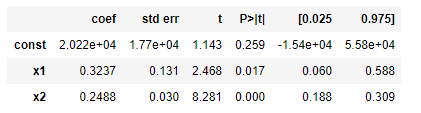
Now, we can see all the variables have p-values less than the significance level. With these variables, we will build the prediction model.

First, divide the new matrix into training and test sets

#Splitting the dataset into the Training set and Test set
from sklearn.model_selection import train_test_split
X_train, X_test, y_train, y_test = train_test_split(X_pred, y, train_size = 0.8, test_size = 0.2, random_state = 0)

Again fit the multiple linear regression model with training set

# Fitting Multiple Linear Regression to the Training set 
from sklearn.linear_model import LinearRegression 
regressor = LinearRegression() 
regressor.fit(X_train, y_train)

Now, predict the value

#Predicting the Test set result 
y_pred = regressor.predict(X_test)

Let's measure the accuracy to see whether we could improve the model

from sklearn.metrics import mean_squared_error 
print("The Mean Squared Error is- {}".format(mean_squared_error(y_test, y_pred))) 

The Mean Squared Error is- 1846130824.0073693

Wow! We made it! The mean absolute error has come down to 18%. So, the backward elimination method is very much helpful to build better multiple linear regression models.

Final Words

In this tutorial, I have tried to explain all the important aspects of multiple linear regression. The key takeaways of the tutorials are-

• What is multiple linear regression
• Implementing multiple linear regression in Python
• Understanding different methods to improve the performance of a multiple linear regression model
• Implementing the backward elimination method

Hope this tutorial helped you to understand all the concepts. If you have any questions or suggestions about the tutorial, please let me know in the comments.

Happy Machine Learning!