Autoencoder | Deep Learning

An autoencoder is a type of Unsupervised Learning in Deep Learning that is designed to learn the compact, lower-dimensional representations of input data by minimizing the reconstruction loss. The autoencoder is used to compress the data and reduce its dimensionality. This Neural network can learn to reconstruct images, text, and other data from compressed versions of themselves.        

Autoencoder plays a significant role in Deep Learning. It is used for many purposes. Some of them are listed below:

• Dimensionality Reduction: It can reduce the dimensionality of input data that is needed for visualizing high dimensional data, reducing computation complexity and mitigating the curse of high dimension in Deep Learning tasks.

• Feature Learning: It can learn the meaningful, important features from input data, which can be used in Machine Learning Algorithms or Fully connected layers in Neural Networks for Classification, regression, or other tasks.

• Denoising: It can be used to remove noise from data that is useful in image processing and audio processing, where noise degrades the quality of data.

• Anomaly Detection: It can be used to detect anomalies from input data by measuring the reconstruction error. While the reconstruction error becomes high, means a potential anomaly.

• Data Generation: Some autoencoder variants can generate new data samples from latent space, which is useful in image synthesis, drug discovery, and so on.

• Representation Learning: It can learn abstract, hierarchical representations of input data that are important for understanding complex data patterns and relationships.

• Image inpainting: It can be used to fill the missing or corrupted part of the image by learning the structure and patterns of the data.

• Text generation: Some Generative autoencoder variants can be used to generate new text samples from the learned latent space.

• Pretraining for NLP task: It can be used for unsupervised pretraining of models such as sentiment analysis, named entity recognition, machine translation, and so on. 

There are a lot of applications with respect to Autoencoder such as Image Compression, text denoising, Unsupervised anomaly detection, semi-supervised anomaly detection, and so on. 

Understanding Autoencoders

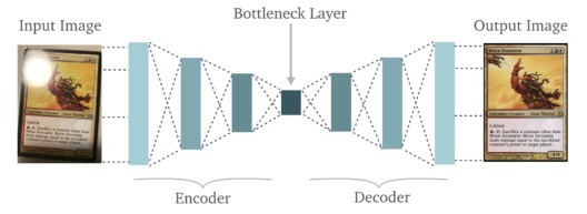
Generally, Autorencoders encode the input data into a lower dimensional representation, then reconstruct the lower dimensional data into Original Data as closely as possible.

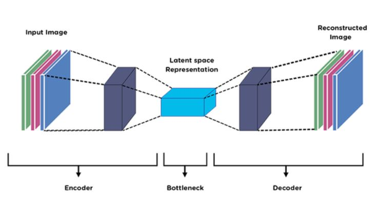
There are three main components in Autoencoder. A brief explanation of those components is given below:

• Encoder: It is a type of Neural Network that can be made by Fully connected layers, Convolutional Layers, Recurrent Layers, and other layers. It takes the input data and then captures the important features/information from the input data and reduces the unnecessary details. Overall, After taking input data, it converts the data into lower dimensional representations which contain the only important features and removes the unnecessary features.

• Bottleneck: The encoder converts the input data into lower dimensional representations that are called the Bottleneck or latent space representations. It is a compressed form of input data that contains the important features of input data. It serves as a bridge between the encoder and decoder of the model. If The Bottleneck becomes too small, then the model can be overfit. 

• Decoder: It is another neural network that takes the latent space representations or low dimensional data (comes from the encoder) and then tries to reconstruct the original input as closely as possible. The encoder compresses the input data into lower dimensional representation and Decoder decompresses the lower dimensional representation into original data as close as possible. The architecture of the decoder is often symmetric to the encoder architecture which gradually expands the representations back to the original dimensions. The performance of the decoder is measured by how well it can reconstruct the latent space to the original data.

Overall, the process of Autoencoder is, Encoder takes the input data, compress the data into lower dimension data (latent space representations/bottleneck), then Decoder takes the lower dimension data and attempts to reconstruct the latent space to the original data as close as possible. Hope you can understand the basic concept of AutoEncoder. 

Types of AutoEncoder

There are several autoencoder architectures have been discovered to address various tasks. Some of them are listed below

• Undercomplete Autoencoder: It is one of the simplest types of autoencoders that is an Unsupervised Neural Network. This autoencoder is used to compress the input data which is called dimensionality reduction of input data. The primary goal is to create a compressed form of input data and can reconstruct the compressed data into original data when needed. 

• Sparse Autoencoder:  It is very hard to set a flexible number of nodes in the hidden layers. The sparse autoencoder is controlled by changing the number of nodes at each hidden layer. It works by penalizing the activations of some neurons in hidden layers. The loss function of the sparse autoencoder calculates the number of neurons that have been activated and provides a penalty that is directly proportional to that. This is called sparsity function which prevents the neural networks from activating more neurons and acts as a regularizer. A typical regularizer creates a penalty on the weights of the nodes, while a sparsity regularizer penalizes the number of nodes activated. Because of the sparsity function, It is not needed to worry about the set dimension of the bottleneck(latent space). There are two ways that can include in the loss function as a sparsity regularizer term. Including 

• L1 Loss 

• KL Divergence Method

• Contractive Autoencoder: It introduces an additional regularization term in the loss function that encourages the learned latent representation to be robust. This can happen by penalizing the Frobenius norm of the Jacobian matrix of the encoder’s output with respect to its input. The Jacobian represents the rate of change of the encoder’s output with respect to input changes. 

  Loss = Reconstruction loss + lambda * contractive penalty

  Here, penalizing the contractive penalty in the loss function, It encourages the encoder to learn more smooth and stable latent representations. Denoising data, feature extraction, and representation learning are the applications of Contractive Autoencoder.

• Denoising Autoencoder: This autoencoder is used to remove the noise from the input data. Here, we feed a noisy image or add some noise in the input data into the model and let it map the lower dimensional manifold that filters out the noise from the image. It can be used for image or audio denoising, and robust feature learning. 

• Variational Autoencoders (VAEs): It is a generative model that learns a probabilistic latent space representation whereas regular autoencoders learn deterministic latent space. In VAEs, the encoder maps the input data into a probability distribution. Then it introduces a sampling step instead of directly using latent representations. Then decoder takes sampled latent space and reconstructs the input data. By taking the sampled latent space, Decoder can reconstruct the input data as well as generate new data samples. It consists of two terms in the loss functions (reconstruction loss and regularization term). The regularization term is KL(Kullback Leibler) divergence which encourages the learned distribution in the latent space to be close to the prior distribution. Data generation, Image synthesis, Anomaly detection, and drug discovery are some applications of VAEs.

• Stacked Autoencoder: It is a deep autoencoder that consists of multiple layers of encoders and decoders stacked on top of each other. It is used to learn hierarchical representations of the input data by training each layer in a layer-wise manner. It can capture more complex patterns and structures of the input data. Denoising, Data Compressor, and Feature extraction is some applications of Stacked Autoencoder.

• Convolutional Autoencoder: It uses convolutional layers in both the encoder and decoder instead of using fully connected layers. It is well suited to grid-like data(images). It can learn local patterns and hierarchical representations in an efficient manner rather than a regular autoencoder. Here reconstruction error(mse or cross-entropy loss) is used as the loss function. Image denoising, feature extraction, Image inpainting, Dimensionality reduction, and Anomaly Detection are some examples of Convolutional Autoencoders.

• Sequence to Sequence Autoencoder: A Seq2Seq Autoencoder is designed to handle sequential data like time series analysis, and natural language processing. In both encoder and decoder architecture, this autoencoder consists of Recurrent Neural Networks(RNN) or other sequential architectures like LSTMs, GRUs, Transforms, and so on. This autoencoder is special for handling sequential data. Denoising, Anomaly detection, and Dimensionality reduction are some applications of Seq2Seq Autoencoder.

• Generative Adversarial Networks(GANs): It is a generative model with a different structure and training mechanisms compared to Autoencoders. Mainly it has two parts(Generator & Discriminator). The generator tries to generate new data samples and Discriminator tries to classify the given samples(fake or real). Image synthesis, Colorization, Image style transfer, and Data augmentation are some applications of GANs.

The number of autoencoder types increasing day by day. There are other autoencoders that are used in specific terms and play a significant role in Deep Learning applications.

AutoEncoder Implementation with CIFER-10 Dataset

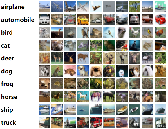
Today we will implement the Autoencoder model with the CIFER-10 dataset. The CIFER-10 dataset is a widely used dataset that contains 60000 images with 32*32 size divided into 10 classes. Each class consists of 6000 images. We will take images, then compress the data by the encoder, then decompress the latent space into original images as closely as possible by the decoder. At the last, we will see the original images and reconstruct images.

Let's see some images of each class of the CIFER-10 dataset.

Tensorflow

At first, some necessary libraries are imported to implement the Autoencoder with CIFER-10 Dataset. The Cifer10 dataset is taken from the Keras dataset library. Conv2D is for an encoder model that compresses the input data and Conv2DTranspose is for a decoder that decompresses the latent space into original input data. Flatten for converting the data into a 1D vector. Dense is for fully connected layers. Reshape is for reshaping the data and Model is for creating the Autoencoder model. Y0u will get the code in Google Colab also.

# import the required packages
import tensorflow as tf
from tensorflow.keras.layers import Conv2D, Conv2DTranspose, Input, Reshape, Flatten, Dense
from tensorflow.keras.models import Model
from tensorflow.keras.datasets import cifar10
import numpy as np

Load Data and Normalize

CIFER-10 data is taken as training and testing data where training data consists of 50000 samples and 10000 images for test data. Then normalize the value of the training & testing data into (0 to 1). 

# Load and preprocess the CIFAR-10 dataset
(x_train, _), (x_test, _) = cifar10.load_data()
x_train = x_train.astype('float32') / 255.0
x_test = x_test.astype('float32') / 255.0

Create Autoencoder Model

To create an autoencoder model, need to create two main parts (Encoder & Decoder). First, define the shape of the input data.

 Then Encoder takes two Convolutional layers and two pooling layers. Convolutional layers consist of 32 & 64 filters with (3*3) kernel_size and Relu activation functions. Max pooling with (2,2) window size for two times is used as pooling layers to reduce the dimensionality of the feature map that comes from the convolutional layers. 

Then Decoder takes the latent space that is generated from the encoder. It takes Transpose Convolution (Conv2DTranspose) 3 times for deconvolution and Upsampling is used which is the inverse of pooling methods 2 times. Conv2DTranspose takes 32 & 64 filters with (3*3) kernel_size and last Conv2DTranspose is using 3 filters for 3 channels of image. Then create the autoencoder model by Keras Model Object that connects the input and output. 

Then compile the model with the ‘adam’ optimizer and ‘mse’ loss function for reconstruction loss.

# Define the autoencoder architecture
def autoencoder():
    input_img = Input(shape=(32, 32, 3))
    # Encoder model that compress dataset
    x = Conv2D(32, (3, 3), activation='relu', padding='same')(input_img)
    x = tf.keras.layers.MaxPooling2D((2, 2), padding='same')(x)
    x = Conv2D(64, (3, 3), activation='relu', padding='same')(x)
    x = tf.keras.layers.MaxPooling2D((2, 2), padding='same')(x)
    # Decoder model that reconstructs the compressed data into original format
    x = Conv2DTranspose(64, (3, 3), activation='relu', padding='same')(x)
    x = tf.keras.layers.UpSampling2D((2, 2))(x)
    x = Conv2DTranspose(32, (3, 3), activation='relu', padding='same')(x)
    x = tf.keras.layers.UpSampling2D((2, 2))(x)
    decoded = Conv2DTranspose(3, (3, 3), activation='sigmoid', padding='same')(x)

# define the autoencoder model
autoencoder = Model(input_img, decoded)
autoencoder.compile(optimizer='adam', loss='mse')
return autoencoder

Train the Autoencoder Model

Our model is ready to train. Autoencoder takes the input & output same. Epochs are taken as 100. Test data is taken as validation data. Batch size defines the number of samples that will be used for each update of the model weights. 

After training the model, at the last epoch we get a training loss is 0.0013 and a validation loss is 0.0013. That is called a reconstruction error. Our model can be learned well and no overfitting has occurred.

# Create the autoencoder model
model = autoencoder()
# Train the autoencoder
model.fit(x_train, x_train,
          epochs=100,
          batch_size=128,
          shuffle=True,
          validation_data=(x_test, x_test))

After performing 100 epochs of the model, the model gives the result like below. Here last 5 epochs are shown to understand the performance of the model during training.

Epoch 95/100
391/391 [==============================] - 4s 9ms/step - loss: 0.0013 - val_loss: 0.0013
Epoch 96/100
391/391 [==============================] - 4s 9ms/step - loss: 0.0013 - val_loss: 0.0013
Epoch 97/100
391/391 [==============================] - 4s 10ms/step - loss: 0.0013 - val_loss: 0.0012
Epoch 98/100
391/391 [==============================] - 4s 9ms/step - loss: 0.0013 - val_loss: 0.0013
Epoch 99/100
391/391 [==============================] - 4s 9ms/step - loss: 0.0013 - val_loss: 0.0013

Predict and Visualize Original & predicted Images

The model has already been trained. Now it is needed to see, how well the model can reconstruct with the test data. So, here we predict the model with test data. Then Visualize the original images along with the predicted images that is reconstructed by the model.

# Test the autoencoder
decoded_imgs = model.predict(x_test)
n = 10  # Number of images to display
plt.figure(figsize=(20, 4))
for i in range(n):
    # Display original
    ax = plt.subplot(2, n, i + 1)
    plt.imshow(x_test[i])
    plt.title("Original")
    plt.axis('off')
    # Display reconstruction
    ax = plt.subplot(2, n, i + 1 + n)
    plt.imshow(decoded_imgs[i])
    plt.title("Reconstructed")
    plt.axis('off')
plt.show()

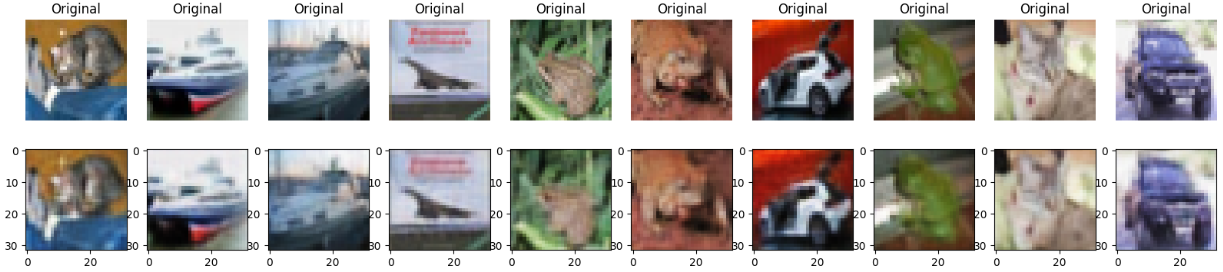
Overall, the TensorFlow model can learn the features correctly and reconstruct the images so nicely. 

Pytorch

First import some necessary libraries to create the autoencoder model and train with training data. Torch.nn is taken for layers, activation function, loss function, and others. Torch.optim is used for optimization technique. Torchvision library provides datasets, pre-trained models, and others. DataLoader is used to load the data in a efficient way with batch size, parallelization, and so on and matplotlib library is for visualization.  

import torch
import torch.nn as nn
import torch.optim as optim
import torchvision
from torchvision import datasets, transforms
from torch.utils.data import DataLoader
import matplotlib.pyplot as plt

Data Loading and Preprocessing

Transform methods converts the PIL image into a tensor that is applied at the time of taking CIFAR10 dataset from torchvision dataset. After taking the dataset as a train dataset and test dataset, Load the dataset into DataLoader functions where the batch size is 128 and the number of workers is 2 as parallelization. 

# Data preprocessing
transform = transforms.Compose([
    transforms.ToTensor()
])
# Load and preprocess the CIFAR-10 dataset
train_dataset = datasets.CIFAR10(root='./data', train=True, download=True, transform=transform)
test_dataset = datasets.CIFAR10(root='./data', train=False, download=True, transform=transform)
train_loader = DataLoader(train_dataset, batch_size=128, shuffle=True, num_workers=2)
test_loader = DataLoader(test_dataset, batch_size=128, shuffle=False, num_workers=2)

Create Autoencoder Model

In Autoencoder, there are two main parts (Encoder and Decoder). Encoder is used to compress the data and Decoder decompresses data and tries to reconstruct the original image as closely as possible.

In Encoder, Convolutional layers are taken two times where the first layer takes input 3 (channel of input data), output 32 filters,(3*3) kernel size, and padding is 1, and 2nd convolutional layer takes 32 input and provides 64 output filters. Relu is taken as an activation function and Maxpool is taken for reduced dimensionality where the window size is (2*2). By encoder, the model makes the latent space of the input data.

Then Decoder, The 2D transpose Convolution (deconvolutional) decompresses the latent space and upsamples the compressed data and the last output of convTranspose2D is 3 which is a channel of the input image.

Then Forward method defines the forward pass of the autoencoder. The encoder takes the input and the decoder returns the reconstructed image. 

# Define the autoencoder architecture
class Autoencoder(nn.Module):
    def __init__(self):
        super(Autoencoder, self).__init__()
        # Encoder
        self.encoder = nn.Sequential(
            nn.Conv2d(3, 32, 3, padding=1),
            nn.ReLU(inplace=True),
            nn.MaxPool2d(2, 2),
            nn.Conv2d(32, 64, 3, padding=1),
            nn.ReLU(inplace=True),
            nn.MaxPool2d(2, 2)
        )
        # Decoder
        self.decoder = nn.Sequential(
            nn.ConvTranspose2d(64, 32, 4, stride=2, padding=1),
            nn.ReLU(inplace=True),
            nn.ConvTranspose2d(32, 3, 4, stride=2, padding=1),
            nn.Sigmoid()
        )
    def forward(self, x):
        x = self.encoder(x)
        x = self.decoder(x)
        return x

Define loss and Optimization Technique

If a ‘cuda’ capable GPU is available, The device can use it otherwise the device will use a CPU. Then create the instance of the Autoencoder model. Then define the mean square loss(mse) for the reconstruction task and ‘adam’ is for the optimizer where the learning rate is 0.003.

# Create the autoencoder model
device = torch.device("cuda" if torch.cuda.is_available() else "cpu")
model = Autoencoder().to(device)
criterion = nn.MSELoss()
optimizer = optim.Adam(model.parameters(), lr=1e-3)

Train the Model

Now, train the model with 100 epochs. At first, forward pass are happen by model(img). Then compute the loss function. Then clear the gradients of all variables and compute the loss with respect to the model’s parameter. Then update the model’s parameter and print the result with the reconstruction loss of each epoch.

After training the autoencoder model with 100 epochs, the last 5 epochs loss is shown which is almost 0.0014. 

# Train the autoencoder
num_epochs = 100
for epoch in range(num_epochs):
    for data in train_loader:
        img, _ = data
        img = img.to(device)
        output = model(img)
        loss = criterion(output, img)
        optimizer.zero_grad()
        loss.backward()
        optimizer.step()
    print(f'Epoch [{epoch + 1}/{num_epochs}], Loss: {loss.item():.4f}')
Epoch [94/100], Loss: 0.0015
Epoch [95/100], Loss: 0.0013
Epoch [96/100], Loss: 0.0013
Epoch [97/100], Loss: 0.0014
Epoch [98/100], Loss: 0.0014
Epoch [99/100], Loss: 0.0015
Epoch [100/100], Loss: 0.0014

Evaluate the model and Visualization

model.eval() means the model is in evaluation mode, which disables features like Drop out, Batch Normalization, and so on. ‘Torch.no_grad’ indicates the gradient computation is disabled during the test phase. Then take the test images from the test loader and predict reconstructed images by the trained model. 

After predicting the reconstructed images, the original images as well as the predicted images are shown below.

# Test the autoencoder
model.eval()
with torch.no_grad():
    for data in test_loader:
        img, _ = data
        img = img.to(device)
        output = model(img)
        # Visualize the results
        if torch.cuda.is_available():
            img = img.cpu()
            output = output.cpu()
        n = 10  # Number of images to display
        plt.figure(figsize=(20, 4))
        for i in range(n):
            # Display original
            ax = plt.subplot(2, n, i + 1)
            plt.imshow(torchvision.utils.make_grid(img[i], nrow=1).permute(1, 2, 0))
            plt.title("Original")
            plt.axis('off')
            # Display reconstruction
            ax = plt.subplot(2, n, i + 1 + n)
            plt.imshow(torchvision.utils.make_grid(output[i], nrow=1).permute(1, 2, 0))
            plt.title("Predicted")    
    plt.show()

The output of the original images and reconstructed images are given below for better understanding.

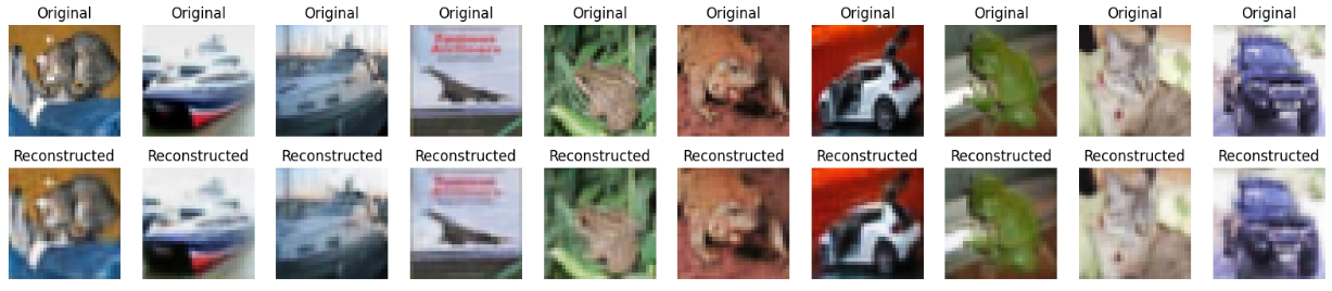
Finally, the Pytorch model can learn the features correctly and reconstruct the images so well. 

Frequently Asked Questions

Autoencoder is a popular technique in the deep learning area. As increasing popularity, the questions with respect to Autoencoders is increasing day by day. Some of the questions are given below:

What is the difference between Autoencoder and PCA(Principal Component Analysis)?

PCA and Autoencoder both are used as dimensionality reduction techniques. But PCA can understand the linearity of the data and Autoencoder can understand the non-linearity of the data. Autoencoder can capture the complex patterns or relationships of the data, whereas PCA can only capture the linear relationships of the data. PCA is computationally efficient and easy to interpret whereas Autoencoder is computationally expensive. Autoencoder gives better performance than PCA. 

How does an AutoEncoder work?

It compresses the input data into lower dimensional space(latent space/bottleneck) and then decompress the lower dimensional data into the original dimension. Its main goal is to reconstruct the input image by minimizing the reconstruction error. 

What does reconstruction error mean in Autoencoder?

It refers to the difference between the original input data and reconstructed output data by autoencoder. Mean Squared Error(MSE), Cross Entropy loss (when the reconstructed output is categorical) is used as reconstruction error. A low reconstruction error means it can capture meaningful representations of the input data from latent space whereas a high reconstruction error can’t capture the essential features of the input data.

What is the difference between Autoencoder and Encoder-Decoder models?

Autoencoder is a special type of Encoder-Decoder model where input and output are the same as the training phase. On the other hand, the Encoder decoder model can consist of different inputs and outputs at the time of the training phase.

When should Autoencoder be used rather than Principal Component Analysis(PCA)?

When the data is complex (image, audio, text, or raw data), and contains non-linear relationships then autoencoder is the best option to use and perform dimensionality reduction.

What are the uses of Autoencoders?

There are several uses of autoencoders such as Data Compression, Dimensionality Reduction, Feature Extraction, Denoising Data, Anomaly Detection, Image inpainting, Generating new data samples (VAEs), Image to Image translation, Sequence to Sequence learning and so on.

What is the role of the activation function in Autoencoder?

The activation function helps the model to introduce non-linearity. In Autoencoder, we can capture complex, non-linear relationships because of activation functions. 

Which AutoEncoders are used to generate new data samples?

Generally, two types of autoencoders are used in this perspective such as Variational Autoencoders, and Adversarial Autoencoders. VAEs learn the probabilistic representation of the input data in the latent space and generate new samples by sampling from the learned distribution. On the other hand, Adversarial Autoencoder adds an adversarial part to the general autoencoder. GANs(Generative Adversarial Networks) are a type of Adversarial Autoencoder.

What are the different activities in the latent space of Variational Autoencoder(VAEs) and regular autoencoder?

VAEs learn probabilistic distribution in the latent space, which means here encoder maps the input data to a probability distribution such as Gaussian. Where regular Autoencoder learns deterministic distribution in the latent space, which means the encoder maps the input data to a specific point in the latent space.

How can Autoencoders identify the anomalies in the data?

Autoencoders will reconstruct the normal data with low reconstruction error and for an anomaly, it gives high reconstruction error. So, it can detect anomalies when the model gives a high reconstruction error.

Cool. You have learned a lot of things about Autoencoders. Hope you can gather a lot of knowledge in the term of Autoencoder and enjoy the article.