Variational Autoencoders | Deep Learning

Autoencoders are an unsupervised learning technique that can learn the efficient representation of input data and are used for various purposes such as dimensionality reduction, data compression, data reconstruction, anomaly detection, denoising, generative modeling and so. General autoencoders use deterministic mappings from the input data to the latent space so that they can’t generate new data samples while Variational Autoencoders(VAEs) introduce probabilistic mapping in the latent space which enables the model to generate new data samples. Also, VAEs can handle other applications of autoencoder as well as generate new data samples. Today you will learn the VAEs deeply that can be used in many use cases. Let’s get started.

Before deep dive into the details of the tutorial, let’s know the concept of the tutorial. The tutorial will be divided into six parts. They are:

• Introduction

• The structure of autoencoder and how it works

• Loss functions 

• VAEs implementation

• Generating new data samples & visualization

• Conclusion

Introduction

Variational autoencoders(VAEs) is a generative model that can learn the probabilistic mapping from the input data and enable the model to generate new data samples. VAEs encode the high dimensional data to the lower dimension in the latent space while latent space is a form of probabilistic distribution. Then the decoder reconstructs the input data from the samples in the latent space. VAEs enforce a regularization on the latent space that encourages the learned latent space to be close to chosen prior distribution(generally standard normal distribution). To generate new data samples, we first draw random points from the prior distribution in the latent space. Then pass them to the trained decoder model that is responsible to generate new data samples. 

Applications of Variational Autoencoders

Variational autoencoders are a type of autoencoders that uses probabilistic mapping from the input image in the latent space instead of deterministic mapping. It has the ability to perform the applications of autoencoders as well as generate new data samples. Some applications of VAEs are given below.

• Generative modeling: It can generate new, realistic samples of any type of data (images, text, audio, other) based on the learned distribution of the trained data.

• Data Compression: It can achieve a good compression ratio as well as the quality of the reconstructed data.

• Anomaly detection: It can be used in anomaly detection by measuring the reconstruction error of the new data samples. If the sample gives a high reconstruction error, then it will consider anomalous otherwise not.

• Image denoising: It can be used to remove noise and reconstruct clean images from noisy images. 

• Dimensionality reduction: It has the ability to reduce the dimension of the input data and visualize the high dimensional data. It can provide insights into the underlying structure of the data.

• Molecular Generation: By learning the probabilistic continuous latent space for molecular structures, It can generate new molecules with desired properties. 

• Data Augmentation: It can generate new data samples that can be used as a data augmentation technique.

• Video Generation: It can be used to learn the sequence, structure, and dynamics of the video data and generate new video sequences. Many applications such as animation, video game design, and simulating realistic environments can be done by VAEs.

Actually, there are a lot of applications that exist with respect to variational autoencoders where some popular items are discussed. The number of applications is increasing and the research on this topic is ongoing. 

Structure & Working Process of VAEs 

Variational autoencoders is a generative model that learns the probabilistic mapping from input data consisting of two main parts such as encoder & decoder. The encoder encodes the high dimensional data into latent space where the decoder neural network decodes the sample(comes from latent space) and generates a new data sample. A brief explanation is given below.

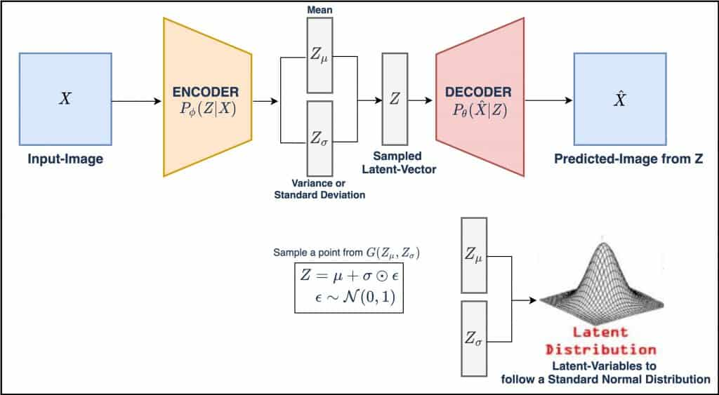
• Encoder: The encoder network maps the input data to parameters of a probability distribution in the latent space. Simply this network takes the input data and processes it through a series of layers ( such as fully connected layers, convolutional layers, recurrent layers, and so on) and gives a set of parameters that define the posterior distribution of the latent vectors. The Encoder is used to learn the approximate posterior distribution of the latent vectors based on a given input sample.

• Latent Space: It is the output of the Encoder network that is a lower dimensional representation of input data. Generally, the VAEs model learns the probabilistic mapping between the input data and latent space. Because of probabilistic distribution on the latent space, VAEs allow the model to generate new data samples. 

• Distribution Parameters: It is a set of parameters of the probability distribution in the latent space. For Gaussian Distribution, The parameters are mean & Log variance. Those are used to define the distribution from which the latent vectors are sampled.

• Regularization: Kullback-Leibler (KL) divergence is used as a regularization technique in the loss function that encourages the learned latent distribution to be close to a chosen prior distribution. This leads to more structured latent space and improves generative capabilities. 

• Reparameterization Trick: This trick is used for training VAEs. It allows gradients to flow through the random sampling step in the latent space which is required to optimize the model’s parameters. To generate a new data sample, at first, we need to draw a random point from the parameters(mean, variance). This direct sampling operation is nondifferentiable and impossible to backpropagate gradients through it. The reparameterization trick solves the problem by separating the deterministic and stochastic components of the sampling operation. Instead of directly sampling from the learned distribution, at first it is needed to sample an auxiliary noise variable from a standard normal distribution and then transform this noise variable using learned parameters from the encoder.

  z = μ + σ ⊙ ε

  Now z is the sample from the learned distribution where mean & variance is the parameters of the encoder and epsilon is the auxiliary noise variable. This transformation is now differentiable with respect to the parameters of the learned distribution. Overall, the reparameterization trick is an essential technique that is responsible for training VAEs by separating the stochastic(random epsilon) and deterministic(non-random mean & variance) variables and making the sampling operation differentiable and gradient-based optimization in VAEs.

• Decoder: The decoder model takes the sample from the latent space and reconstructs the original input image. The decoder neural network is a type of neural network that may be fully connected to dense layers, Deconvolution, or recurrent neural network. The encoder compresses the input data into lower dimensional data and decoder reconstructs the lower dimensional data into the original data dimension. 

The overall process of VAEs is encoder neural network takes the input data and produces a probability distribution in the latent space. The distribution parameters are mean & variance. Then reparameterization trick helps the model to train with gradient-based optimization in the probability distribution. Then decoder takes the sample from probability distribution in the latent space & reconstructs the sample into the original image dimension. Then the loss function is calculated between the generated data sample and the actual data sample. During the training VAEs, it optimizes the evidence lower bound (ELBO) which includes the reconstruction loss and the KL divergence. Thus VAEs are capable of generating new data samples by sampling from the prior distribution in the latent space by passing the samples in the trained decoder network.

Loss Function in VAEs

To understand the performance of the VAEs model, It is needed to clear the concepts of loss function used in VAEs. We know that during training, VAEs optimize the evidence lower bound (ELBO) which includes reconstruction loss and regularization term (Kullback Leibler(KL) divergence). During training, the goal of the VAEs model is to minimize the sum of these two components. The details are given below.

Reconstruction Loss

It measures how well the VAEs model can reconstruct the input data from the latent space representation. It calculates the difference between the original input and the reconstructed output. The reconstruction loss function can be different based on types of the data.

• Mean Squared Error (MSE) can be used as reconstruction loss for continuous data. It calculates the average squared difference between the original input and reconstruction output.

• Binary Cross Entropy(BCE) for binary data and categorical cross entropy(CCE) for multiclass data can be used whether it measures the dissimilarity between the true labels and predicted labels.

Kullback-Leibler (KL) divergence

It is used as a regularization term that enforces a specific structure on the latent space. It measures the difference between the learned latent distribution(mean & log variance) and a chosen prior distribution(a standard normal distribution). Its goal is to goal minimize the KL divergence that pushes the learned latent distribution to be close to the prior distribution and make a more structured and smooth latent space.

At the time of training the VAEs model, it minimizes the ELBO loss function to learn an optimal mapping between the input data and the latent space. Balancing the reconstruction loss and KL divergence is essential. Because if reconstruction loss is too dominant, the model may overfit and fail to learn a structured & smooth latent space. Otherwise, if the KL divergence is too dominant, the model may generate samples that do not resemble the original data distribution. So, careful notice is needed in the loss function at the time of training VAEs.

Implement the Variational Autoencoders Model

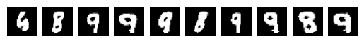
Today you can learn the variational autoencoders (VAEs) implementation in python with the MNIST dataset. MNIST dataset is a popular dataset for computer vision tasks. It consists of 70000 images of digits and it labels also where 60000 images are for training and 10000 images are for testing the model. It is a collection of grayscale images with (28*28) size. Now first we will train our variational autoencoder model with a training dataset and then generate new data samples by predicting test data and at last, you can see the interpretation as well as visualization of latent space representations of the VAE model. Let’s get started.

Tensorflow

Firstly import the necessary libraries to perform the implementation. ’Matplotlib’ is for visualization of the generated output and latent space and ‘Tensorflow’, ’keras’ are for building models and implementing with mnist dataset. You will get the code in Google Colab also.

import matplotlib.pyplot as plt
import numpy as np
import tensorflow as tf
from tensorflow import keras
from tensorflow.keras import layers

Load Data & Preprocess Data

We take the MINST dataset from keras Dataset library. Then combine the train images and test images into mnist_digits variable. Now the size of the images is (28*28). So, adding channels as 1 is performed and normalize the data by dividing 255. Now the data shape is (28*28*1) and normalized. 

(x_train, _), (x_test, _) = keras.datasets.mnist.load_data()
mnist_digits = np.concatenate([x_train, x_test], axis=0)
mnist_digits = np.expand_dims(mnist_digits,-1).astype("float32") / 255

Sampling Layers

The purpose of this layer is to provide a sample of latent space representations from the approximate posterior distribution. The encoder gives the two output mean and log variance. Then batch size and dimension are calculated from the shape of the mean value. Epsilon indicates a random noise that is injected into the sampling process. Then finally return the samples latent space representations using the reparameterization trick.

class Sampling(layers.Layer):
    def call(self, inputs):
        z_mean, z_log_var = inputs
        batch = tf.shape(z_mean)[0]
        dim = tf.shape(z_mean)[1]
        epsilon = tf.keras.backend.random_normal(shape=(batch, dim))
        return z_mean + tf.exp(0.5 * z_log_var) * epsilon

Encoder Model

The dimension of the latent space is defined as 2. The encoder network consists of fully connected layers, and convolutional layers, and finally provide outputs of mean, log variance, and sample latent space representations. At last, the encoder summary has shown to see the parameters of the model.

latent_dim=2
encoder_inputs=keras.Input(shape=(28,28,1))
x=layers.Conv2D(32,3,activation="relu",strides=2,padding="same")(encoder_inputs)
x=layers.Conv2D(64,3,activation="relu",strides=2,padding="same")(x)
x=layers.Flatten()(x)
x=layers.Dense(16,activation="relu")(x)
z_mean=layers.Dense(latent_dim,name="z_mean")(x)
z_log_var=layers.Dense(latent_dim,name="z_log_var")(x)
z=Sampling()([z_mean,z_log_var])
encoder=keras.Model(encoder_inputs,[z_mean,z_log_var,z],name="encoder")
encoder.summary()

By the summary of the model, we can see the output shape of each layer. The latent dimension is 2, so the mean, variance & sampling latent space is 2 where the input shape is (28*28*1). The total parameters is 69,076 where all the parameters are trainable.

Model: "encoder"
   Layer (type)                      Output Shape       Param #     Connected to                     
 input_3 (InputLayer)           [(None, 28, 28, 1)]    0                []                               
                                                                                                  
 conv2d_6 (Conv2D)           (None, 14, 14, 32)   320         ['input_3[0][0]']                
                                                                                                  
 conv2d_7 (Conv2D)            (None, 7, 7, 64)     18496       ['conv2d_6[0][0]']               
                                                                                                  
 flatten_2 (Flatten)            (None, 3136)                0           ['conv2d_7[0][0]']               
                                                                                                  
 dense_4 (Dense)                (None, 16)                50192       ['flatten_2[0][0]']              
                                                                                                  
 z_mean (Dense)                 (None, 2)                  34          ['dense_4[0][0]']                
                                                                                                  
 z_log_var (Dense)              (None, 2)                 34          ['dense_4[0][0]']                
                                                                                                  
 sampling_1 (Sampling)          (None, 2)              0           ['z_mean[0][0]', z_log_var[0][0]']              
                                                                                                  
==================================================================================================
Total params: 69,076
Trainable params: 69,076
Non-trainable params: 0

Decoder model

The decoder network takes the sample latent space representation as input and generates a reconstructed image with the same dimensions as the original input dimension. This model is the reverse of the encoder where it upsamples the latent space into the original image dimension. The input is the latent dimension (2) and output is the original image dimension(28*28*1). Lastly, the summary of the model has been shown for better understanding.

#decoder model to reconstruct/generate images from latent space
latent_inputs = keras.Input(shape=(latent_dim,))
x = layers.Dense(7 * 7 * 64, activation="relu")(latent_inputs)
x = layers.Reshape((7, 7, 64))(x)
x = layers.Conv2DTranspose(64, 3, activation="relu", strides=2, padding="same")(x)
x = layers.Conv2DTranspose(32, 3, activation="relu", strides=2, padding="same")(x)
decoder_outputs = layers.Conv2DTranspose(1, 3, activation="sigmoid", padding="same")(x)
decoder = keras.Model(latent_inputs, decoder_outputs, name="decoder")
decoder.summary()

Here you can see the output shape of each layer.The total parameters are 65,089 where all are training parameters.

Model: "decoder"
_________________________________________________________________
 Layer (type)                Output Shape              Param #   
=================================================================
 input_4 (InputLayer)        [(None, 2)]               0         
                                                                 
 dense_5 (Dense)             (None, 3136)              9408      
                                                                 
 reshape_2 (Reshape)         (None, 7, 7, 64)          0         
                                                                 
 conv2d_transpose_4 (Conv2DT  (None, 14, 14, 64)       36928     
 ranspose)                                                       
                                                                 
 conv2d_transpose_5 (Conv2DT  (None, 28, 28, 32)       18464     
 ranspose)                                                       
                                                                 
 conv2d_transpose_6 (Conv2DT  (None, 28, 28, 1)        289       
 ranspose)                                                       
                                                                 
=================================================================
Total params: 65,089
Trainable params: 65,089
Non-trainable params: 0
_________________________________________________________________

Variational Autoencoder model

This model is designed to combine the previously defined encoder and decoder models and manage the training process including the computations of the loss functions and optimization process. Firstly we take the encoder and decoder model and then define the loss functions. The train_step function is responsible for training the model. It encodes the input data and produces mean, variance & sample latent space representations, then decode the sample and reconstructs as like as the original image. Then measure the loss and apply backpropagation to compute the gradients namely the optimization process. At last print the three losses between reconstructed image and the original image in each epoch. 

class VAE(keras.Model):
    def __init__(self, encoder, decoder, **kwargs):
        super().__init__(**kwargs)
        self.encoder = encoder
        self.decoder = decoder
        self.total_loss_tracker = keras.metrics.Mean(name="total_loss")
        self.reconstruction_loss_tracker = keras.metrics.Mean(
            name="reconstruction_loss"
        )
        self.kl_loss_tracker = keras.metrics.Mean(name="kl_loss")
    @property
    def metrics(self):
        return [
            self.total_loss_tracker,
            self.reconstruction_loss_tracker,
            self.kl_loss_tracker,
        ]
    def train_step(self, data):
        with tf.GradientTape() as tape:
            z_mean, z_log_var, z = self.encoder(data)
            reconstruction = self.decoder(z)
            reconstruction_loss = tf.reduce_mean(
                tf.reduce_sum(
                    keras.losses.binary_crossentropy(data, reconstruction), axis=(1, 2)
                )
            )
            kl_loss = -0.5 * (1 + z_log_var - tf.square(z_mean) - tf.exp(z_log_var))
            kl_loss = tf.reduce_mean(tf.reduce_sum(kl_loss, axis=1))
            total_loss = reconstruction_loss + kl_loss
        grads = tape.gradient(total_loss, self.trainable_weights)
        self.optimizer.apply_gradients(zip(grads, self.trainable_weights))
        self.total_loss_tracker.update_state(total_loss)
        self.reconstruction_loss_tracker.update_state(reconstruction_loss)
        self.kl_loss_tracker.update_state(kl_loss)
        return {
            "loss": self.total_loss_tracker.result(),
            "reconstruction_loss": self.reconstruction_loss_tracker.result(),
            "kl_loss": self.kl_loss_tracker.result(),
        }

Compile the model and start training

Firstly the variational autoencoder model is called with encoder and decoder functions. Adam is used for optimization techniques. Lastly, run the VAE model with 30 epochs and 128 batch size. 

# define the VAE model and compile and run the model
vae = VAE(encoder, decoder)
vae.compile(optimizer=keras.optimizers.Adam())
vae.fit(mnist_digits, epochs=30, batch_size=128)

You can see the last 5 epochs consists of the training loss functions. Here the reconstruction loss functions gradually decrease and kl divergence loss fluctuates. 

Epoch 26/30
547/547 [==============================] - 4s 8ms/step - loss: 146.7310 - reconstruction_loss: 140.3688 - kl_loss: 6.5655
Epoch 27/30
547/547 [==============================] - 4s 8ms/step - loss: 146.6334 - reconstruction_loss: 140.2511 - kl_loss: 6.5655
Epoch 28/30
547/547 [==============================] - 5s 9ms/step - loss: 146.8136 - reconstruction_loss: 140.0361 - kl_loss: 6.5773
Epoch 29/30
547/547 [==============================] - 4s 8ms/step - loss: 146.3380 - reconstruction_loss: 139.8402 - kl_loss: 6.5871
Epoch 30/30
547/547 [==============================] - 4s 8ms/step - loss: 146.6426 - reconstruction_loss: 139.7171 - kl_loss: 6.6072

Generating New Data

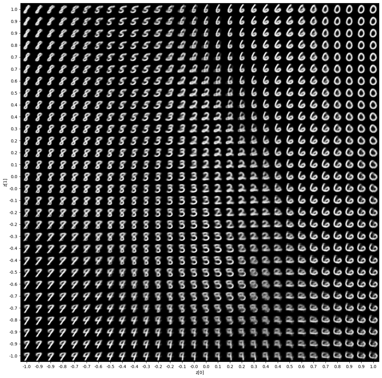
Our model has already been trained. Now it is time to generate new data samples by giving the values in a range of specific scales through the decoder model. Plot_latent_space is a function where trained VAE model, number of samples will generate and fig size is needed. Here we generate n*n digits. In the grid, we take the values from (-scale to scale). For each x and y value, we generate the digits by decoder. Then visualize all the generated images in a graph.

def plot_latent_space(vae, n=30, figsize=15):
    # display a n*n 2D manifold of digits
    digit_size = 28
    scale = 1.0
    figure = np.zeros((digit_size * n, digit_size * n))
    # linearly spaced coordinates corresponding to the 2D plot
    # of digit classes in the latent space
    grid_x = np.linspace(-scale, scale, n)
    grid_y = np.linspace(-scale, scale, n)[::-1]
    for i, yi in enumerate(grid_y):
        for j, xi in enumerate(grid_x):
            z_sample = np.array([[xi, yi]])
            x_decoded = vae.decoder.predict(z_sample)
            digit = x_decoded[0].reshape(digit_size, digit_size)
            figure[
                i * digit_size : (i + 1) * digit_size,
                j * digit_size : (j + 1) * digit_size,
            ] = digit
    plt.figure(figsize=(figsize, figsize))
    start_range = digit_size // 2
    end_range = n * digit_size + start_range
    pixel_range = np.arange(start_range, end_range, digit_size)
    sample_range_x = np.round(grid_x, 1)
    sample_range_y = np.round(grid_y, 1)
    plt.xticks(pixel_range, sample_range_x)
    plt.yticks(pixel_range, sample_range_y)
    plt.xlabel("z[0]")
    plt.ylabel("z[1]")
    plt.imshow(figure, cmap="Greys_r")
    plt.show()
plot_latent_space(vae)

Visualize the latent Space Representation

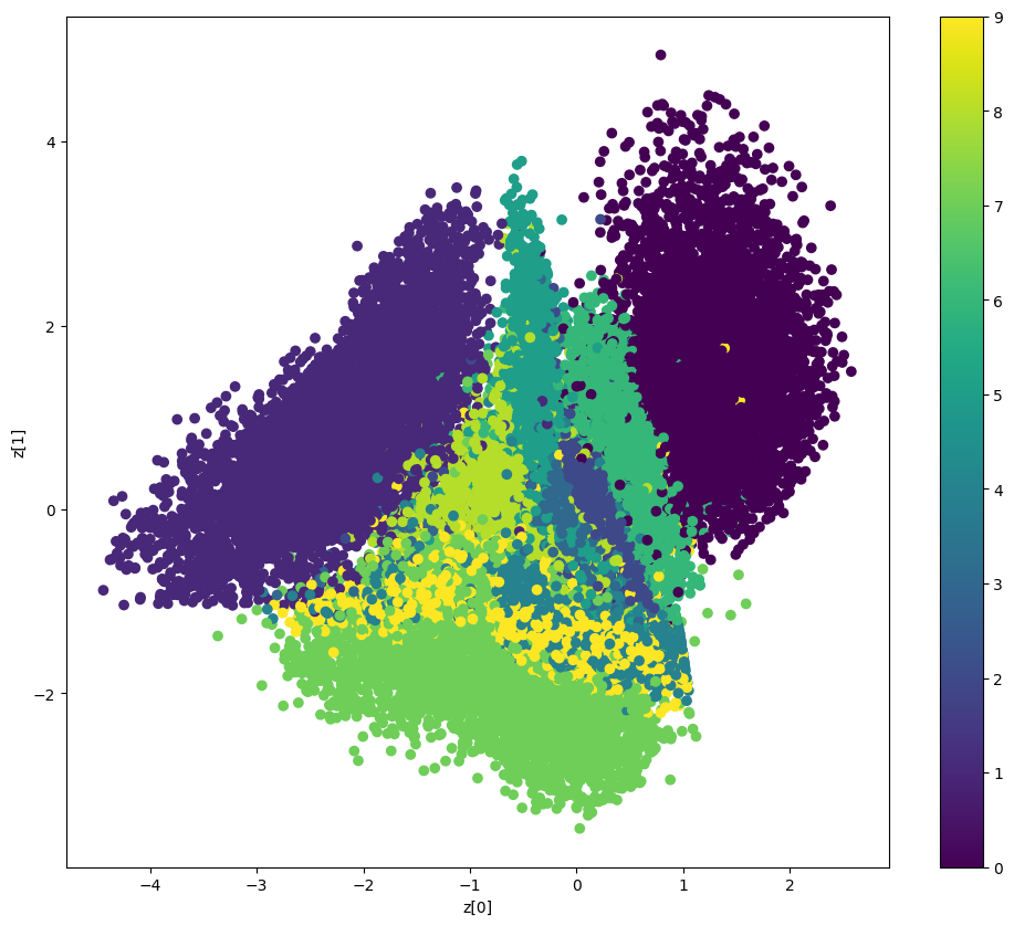
The function defines visualization of the latent space of the trained VAE by generating 2D grid of images. It defines the output of the encoder (mean & variance). So, I take the data and predict the data with the encoder model. Our trained model was 2 dimensions latent space. So, I take the mean value and visualize the scatter points. Below you can see the visualization of the latent space.

def plot_label_clusters(vae, data, labels):
    # display a 2D plot of the digit classes in the latent space
    z_mean, _, _ = vae.encoder.predict(data)
    plt.figure(figsize=(12, 10))
    plt.scatter(z_mean[:, 0], z_mean[:, 1], c=labels)
    plt.colorbar()
    plt.xlabel("z[0]")
    plt.ylabel("z[1]")
    plt.show()
(x_train, y_train), _ = keras.datasets.mnist.load_data()
x_train = np.expand_dims(x_train, -1).astype("float32") / 255
plot_label_clusters(vae, x_train, y_train)

In the graph, the color bar indicates the specific colors for specific digits. The scatter points indicate the digit number for various points. The same color indicates the same digits. In the latent representations, some overlapping has been seen. If the latent space becomes more dimension, then maybe the model can learn better and also need to get the optimal latent dimension. Then you get the accurate latent representations and can avoid the risk of overfitting.

Pytorch

To do variational autoencoder implementation with Pytorch, first import the necessary libraries to perform the task. Here ‘Matplotlib’ is taken for visualization, torch.nn is for model building, optim is for optimization algorithms(Adam), torchvision is a computer vision library that provides various datasets, image transformation, many pre-trained models, and so on. Dataloader class is used for load datasets, handling batching, shuffling, and other parallelization works. 

import torch
import torch.nn as nn
import torch.optim as optim
from torchvision import datasets, transforms
from torch.utils.data import DataLoader
import matplotlib.pyplot as plt

Load Data & Preprocess the Data

The MNIST dataset is taken from the torch-vision dataset library, where transform converts the data into tensor data type & normalizes the images data by giving the mean value 0.1307 & standard deviation value 0.3081. The dataloader makes the training data & testing data suitable by batching and shuffling. Now our dataset is ready for training and evaluation.

# Load and preprocess the MNIST dataset
transform = transforms.Compose([
    transforms.ToTensor(),
    transforms.Normalize((0.1307,), (0.3081,))
])
train_dataset = datasets.MNIST(root='./data', train=True, download=True, transform=transform)
test_dataset = datasets.MNIST(root='./data', train=False, download=True, transform=transform)
train_loader = DataLoader(train_dataset, batch_size=128, shuffle=True)
test_loader = DataLoader(test_dataset, batch_size=128, shuffle=False)

VAE model Creation

This model consists encoder, reparameterization trick & decoder model. The encoder takes the input data and provides the output of mean and log variance with latent dimensions. In other words, encoder is used to learn the parameters (mean & log variance) of the approximate posterior distribution. Here the encoder variable indicates the encoder function. 

Then the reparameterization technique is used to sample the latent variables (z) from the learned distribution. The reparameterize function is responsible for this task which makes the model parameters suitable for optimization. 

Then the decoder function takes the sample from the latent space and reconstructs the sample into original image dimensions. In other words, It is used to generate reconstructed images from the latent variables. 

The forward function defines the forward pass of the variational autoencoder model. This is an overall discussion of the VAE model.

class VAE(nn.Module):
    def __init__(self, latent_dim):
        super(VAE, self).__init__()
        self.latent_dim = latent_dim
        # Encoder
        self.encoder = nn.Sequential(
            nn.Linear(784, 512),
            nn.ReLU(),
            nn.Linear(512, 256),
            nn.ReLU()
        )
        self.fc_mu = nn.Linear(256, latent_dim)
        self.fc_logvar = nn.Linear(256, latent_dim)
        # Decoder
        self.decoder = nn.Sequential(
            nn.Linear(latent_dim, 256),
            nn.ReLU(),
            nn.Linear(256, 512),
            nn.ReLU(),
            nn.Linear(512, 784),
            nn.Sigmoid()
        )
    def reparameterize(self, mu, logvar):
        std = torch.exp(0.5 * logvar)
        eps = torch.randn_like(std)
        return mu + eps * std
    def forward(self, x):
        h = self.encoder(x.view(-1, 784))
        mu, logvar = self.fc_mu(h), self.fc_logvar(h)
        z = self.reparameterize(mu, logvar)
        x_recon = self.decoder(z)
        return x_recon.view(-1, 1, 28, 28), mu, logvar

Define Loss Function & Optimizer

If you have GPU in your device then use that by device variable. The latent dimension is taken as 2. Then call the VAE model into vae. Adam is chosen as the optimizer and reconstruction loss and kL divergence are defined for loss and regularization.

device = torch.device("cuda" if torch.cuda.is_available() else "cpu")
latent_dim = 2
vae = VAE(latent_dim).to(device)
optimizer = optim.Adam(vae.parameters(), lr=1e-3)
def loss_function(x_recon, x, mu, logvar):
    recon_loss = nn.functional.binary_cross_entropy(x_recon, x, reduction='sum')
    kl_loss = -0.5 * torch.sum(1 + logvar - mu.pow(2) - logvar.exp())
    return recon_loss + kl_loss

Train the model

The train function takes the epoch and makes the vae model in train mode by vae.train(). A batch of images is taken from the train loader and then zero the gradients of the optimizer. Then pass the input data into vae model. Then compute the loss function and perform back propagation. And at last print the average loss of each epoch. 

def train(epoch):
    vae.train()
    train_loss = 0
    for batch_idx, (data, _) in enumerate(train_loader):
        data = data.to(device)
        optimizer.zero_grad()
        recon_batch, mu, logvar = vae(data)
        loss = loss_function(recon_batch, data, mu, logvar)
        loss.backward()
        train_loss += loss.item()
        optimizer.step()
    print('Epoch: {} | Average loss: {:.4f}'.format(epoch, train_loss / len(train_loader.dataset)))

After taking epoch as 20, The model started to train and give the losses in each epoch. I just show the last epochs to understand. 

n_epochs = 20
for epoch in range(1, n_epochs + 1):
    train(epoch)
Epoch: 15 | Average loss: -27705.0385
Epoch: 16 | Average loss: -27765.3745
Epoch: 17 | Average loss: -27811.7515
Epoch: 18 | Average loss: -27780.8232
Epoch: 19 | Average loss: -27719.0086
Epoch: 20 | Average loss: -27702.3860

Generate New samples

Here you can see the 10 generated samples. vae.eval() is taken for evaluation mode. No_grad indicates disabled gradient calculations. Then we create some random latent vectors and pass them to a trained decoder model to generate the samples. After generating the samples, The images has shown below. The generated images are almost realistic. 

n_samples = 10
vae.eval()
with torch.no_grad():
    random_latent_vectors = torch.randn(n_samples, latent_dim).to(device)
    generated_images = vae.decoder(random_latent_vectors)
generated_images = generated_images.cpu().view(-1, 28, 28).numpy()
for i in range(n_samples):
    plt.subplot(1, n_samples, i + 1)
    plt.imshow(generated_images[i], cmap='gray')
    plt.axis('off')
plt.show()

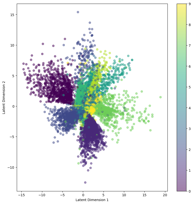
Latent Space Representations

Here you can see the interpretations for latent space for each digit. We evaluate our test data and compute the mean by trained vae model then append those in latent_points. Then scatter plot is shown taking latent points. In the graph, the color bar indicates the specific color for specific digits. So, you can verify the digits by their points. 

vae.eval()
latent_points = []
labels = []
with torch.no_grad():
    for i, (x, y) in enumerate(test_loader):
        x = x.to(device)
        recon_x, mu, logvar = vae(x)
        latent_points.append(mu.cpu().numpy())
        labels.append(y.numpy())
latent_points = np.concatenate(latent_points, axis=0)
labels = np.concatenate(labels, axis=0)
# Plot latent space
plt.figure(figsize=(10, 10))
scatter = plt.scatter(latent_points[:, 0], latent_points[:, 1], c=labels, cmap='viridis', alpha=0.5)
plt.xlabel("Latent Dimension 1")
plt.ylabel("Latent Dimension 2")
plt.colorbar(scatter)
plt.show()

Hope you can understand the implementation of variational autoencoder. Truly, It’s a very basic implementation of VAE. Wish you can explore this knowledge in other applications. 

Frequently Asked Questions about VAEs

Now you can know some extra things about VAEs that is generally asked. It is a very important part that increases the knowledge about VAEs and gathers some extra things that may help in other applications. 

What are the differences between Variational Autoencoders and General Autoencoders?

Variational autoencoders is used to learn a probabilistic mapping between input and latent space instead of deterministic mapping used in vanilla autoencoders. VAEs is capable to generate new data samples over traditional autoencoders. KL divergence regularization is used in VAEs and the reparameterization trick is used to make the sampling process differentiable. These are differences between VAE and autoencoders, the rest are the almost same.

What are the limitations of Variational Autoencoders (VAE)?

It generates less sharp more blurry data samples than other generative models. It may be difficult for a model to learn complex posterior distribution. The choice of objective functions hyperparameter is sensitive. Training on large-scale datasets can be computationally expensive and time-consuming. 

Why Standard Gaussian is used as a prior distribution in the latent variables in VAE?

It is convenient in VAE because of some benefits. Firstly it is mathematically simple and helps the model to regularize the learned latent space. It has a simple reparameterization that enables the model to backpropagate through the sampling process. Also, it is computationally efficient. Anyway, you can choose another distribution but make sure that distribution can handle the hurdles of the VAEs.

Which is the better generative model between GAN and VAE?

The choice of using each generative model depends on the types of tasks. GANs can generate more sharp and more realistic new data samples than VAE. GAN uses complex architectures and performs well in generating new data than VAE. On the other hand, VAE has a more stable training process and easy to interpret the latent representations than GANs. VAE can adopt unsupervised, semi-supervised learning tasks easily where GAN may be complex. So, the use case defines which generative model is better.

How to choose the dimension of the latent variable in VAE?

It depends on the needs of the user and an experimental matter. If the input data is simple or low-dimensional data, then a small latent dimension is sufficient. If the input data is high dimensional, then the latent dimension can be larger to capture the underlying structure of the input data. But it is needed to balance the trade-off between data compression and reconstruction quality. For high-dimensional input data, a small latent variable can be good at data compression but may be poor at the reconstruction of the sample. And a larger latent space can be poor at data compression but good at data reconstruction and also it will increase the risk of overfitting. So optimal latent space dimension is important that can be get by grid search or other experiments and if you have prior knowledge about the underlying structure of the input data, that can be useful in choosing the optimal latent space dimension. 

Does it make sense to use a larger latent space dimension over the input data dimension in VAE?

It is not recommended. Because it diminishes the main advantage of VAE such as dimensionality reduction, learning compact and meaningful latent representations, and generating new data samples. It also increases the risk of overfitting and less interpretable latent representations. 

Are there any benefits of using VAE-GAN instead of just GAN?

Certainly. VAE-GAN is a hybrid model that consists of the advantages of VAE and GAN. It can generate more sharper and realistic samples, the training process is more stable, It encourages the model to make a smooth and interpretable latent space, and flexible for many learning tasks. Overall, this model takes the advantages of the VAE and GAN model and diminishes the limitations of those.

Why do people use MSE for the loss in VAE?

Generally, it is used for continuous value as reconstruct loss function in VAE because of some causes. It is simple and easy to compute. It is a differentiable function that is needed for optimization. It is interpretable and well-suited for continuous data. It imposes a quadratic penalty on errors that focus on reducing larger errors and produce more accurate reconstructions. Because of the many benefits, the use of MSE has increased.

What is the impact of scaling the KL divergence and reconstruction loss in the VAE Objective function?

The VAE objective function acts as a trade-off between KL divergence and reconstruction loss. KL divergence regularizes the latent space that is used to follow a prior distribution. If the weight of KL divergence is increased, then it emphasizes matching the latent space as like prior distribution but may be poor at reconstruction. If it becomes decreased, then the risk of overfitting will increase. Likely, if the weight of reconstruction loss is increased, then the reconstruction quality will increase as well as the complexity of latent space will increase and the regularization will decrease. If the weight of reconstruction loss is decreased, then the quality of reconstruction will decrease. So, to get the optimal balance between two things, scaling plays a very important role. 

What are the types of Variational Autoencoders?

There are many types of VAE including Conditional Variational Auto Encoder (CVAE), Ladder Variational Autoencoder (LVAE), Vector Quantisd Variational Autoencoder (VQ-VAE), Denoising Variational Autoencoder (DVAE), Grammar Variational AutoEncoder (GVAE), Syntax- directed Variational Autoencoder (SD-VAE), PixelVAE, GraphVAE, Constrained Graph Variational Autoencoder (CG-VAE), Character VAE (CVAE), Regularized VAE (RVAE), Junction Tree Variational Autoencoder (JT-VAE) and so on.

What is mode collapse? Why doesn’t VAE suffer mode collapse?

Mode collapse is a common issue in generative modeling where the model fails to capture the diversity of the true data distribution. Instead of generating a variety of samples that represent different modes, the model generates samples that belong to a limited set of modes or even just one mode, indicating the mode collapse. Generally, VAE doesn’t suffer mode collapse because of its objective functions that consist of reconstruction loss and KL divergence Loss. The KL divergence loss prevents mode collapse by encouraging the latent space to follow a smooth distribution and discourage focusing on specific modes in the data. On the other hand, Reconstruction loss ensures the generated samples are similar to the input data. Because of these two components, VAE can capture the diversity of the data and avoid mode collapse.

Hope now you can clarify the concepts and various things about variational autoencoders. The popular questions about variational autoencoder from people have been discussed and hope with this knowledge, you can answer other questions too. 

Conclusion

Today we have covered a lot of things about variational autoencoders(VAEs). You have learned the structure of VAE, applications, implementations of VAEs, and some important discussions about the question answering part. Hope you can gather basic knowledge about VAE and with this knowledge you can explore other applications. Now you can go to the other types of VAEs and can implement them with other datasets with high dimensions and multi-channels. You can make or apply the transfer learning model in VAE. You can make the architecture more complex and can use regularization(early stopping, dropout, and so on), You can try hyperparameter turning such as grid search, random search, and bayesian optimization to get the optimal latent space and model. You can try other metrics for training and evaluation. The experiment is the main thing in Deep Learning. So experiment with the model in a different way. Hope you enjoy this article. Thanks for reading.