Reinforcement Learning in Deep Learning | Deep Learning

Reinforcement Learning (RL) is a machine learning type concerned with how agents learn to interact with an environment to maximize some notion of cumulative reward. In contrast to supervised learning, where the goal is to learn a mapping from inputs to outputs, and unsupervised learning, where the goal is to learn the underlying structure of the data, RL is concerned with learning how to make sequential decisions in an uncertain, dynamic environment.

RL has gained a lot of attention in recent years due to its potential applications in a wide range of fields, including robotics, game AI, and recommendation systems. RL has also been successfully applied to various challenging problems such as playing Atari games, controlling autonomous vehicles, and mastering the game of Go.

In this tutorial, we will discuss the fundamentals of RL, popular RL algorithms, and how to implement RL algorithms with code. We will also explore the applications of RL in deep learning, as well as the challenges and future directions of RL. By the end of this tutorial, you should have a solid understanding of RL and its applications.

Understanding Reinforcement Learning

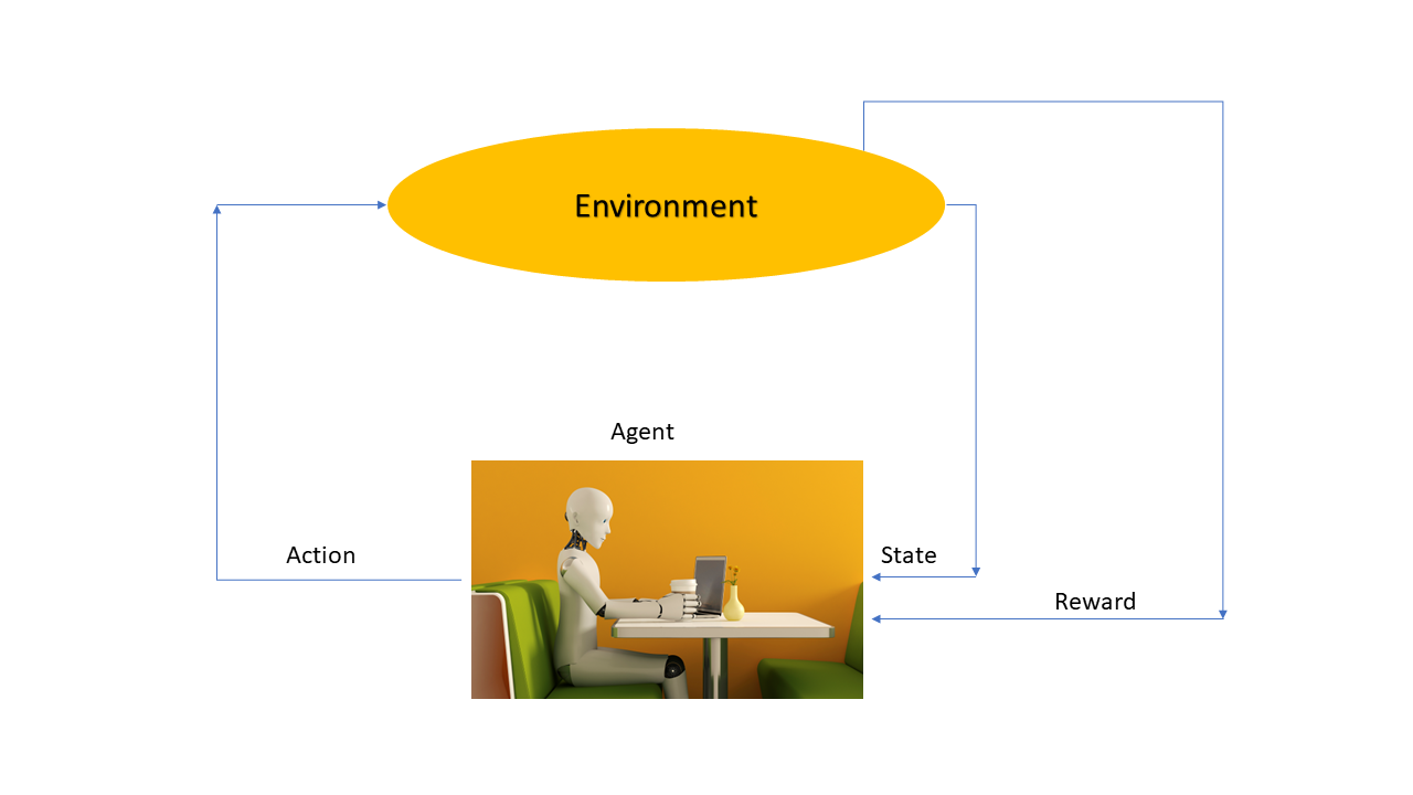
Reinforcement learning is a term used to describe how a robot can learn to make good decisions like the children’s what we teach them in childhood. The robot interacts with its environment and receives feedback through rewards or punishment, which helps it understand which action should happen and which should not.

Think of it like a game board with different squares representing different states. The robot moves around the board, taking action and receiving rewards based on where it lands. The ultimate goal is to teach the robot how to make the best decisions that will lead to the best result.

There are two main types of reinforcement learning: Model-free and model-based.

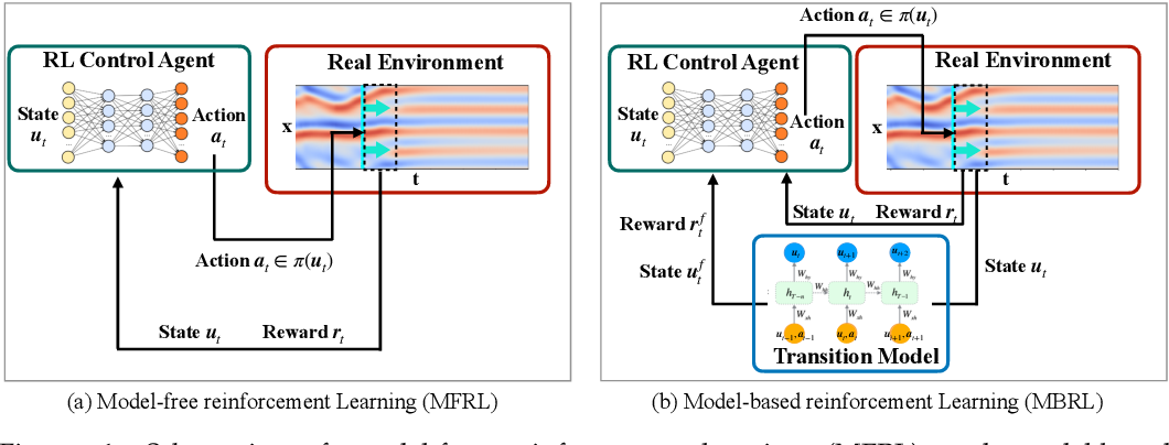
Model-free methods are a way for robots to learn by trial and error, without needing a map of the environment. 

Model-based methods try to learn a model of the environment, which can be pretty slow and requires a lot of resource power. 

RL is like an adventure game where you have to find the best path to get the most treasure. But you have to decide whether to take a new path and explore the unknown or take a path you've already been on to get more treasure. This is the trade-off between exploration and exploitation in RL. Exploration is like trying out new paths to learn more about the game, while exploitation is like using what you already know to get the most treasure. A good RL algorithm should balance these two things so it can learn more about the game while also getting the most treasure possible.

Next, we will discuss some popular RL algorithms.

Reinforcement Learning Algorithms

There are many RL algorithms, each with its own strengths and weaknesses. In this section, we will discuss some popular RL algorithms.

Q-Learning

Q-Learning is a popular reinforcement learning algorithm that enables an agent to learn optimal actions to take in an environment by maximizing cumulative rewards. In the context of Q-Learning, an agent interacts with an environment, receives rewards based on its actions, and aims to learn a policy that guides it to make the best decisions in various states.

Key Concepts of Q-Learning:

Q-Value (Quality Value): The agent keeps a Q-Table that contains the Q-Values for each state-action pair when using Q-Learning. The predicted cumulative reward an agent can get by performing a specific action in a particular state is represented by the Q-Value.

Bellman Equation: The Bellman equation, which updates the Q-Values depending on the rewards received and the future tips anticipated from the next state, is the basis of Q-Learning. It facilitates the agent's iterative Q-Table refinement, resulting in better action choices.

This is the Bellmen’s Equation

                                          V(s) = max[Σ{ P(s'|s, a) * [R(s, a, s') + γ * V(s')]}]

In this equation:

• V(s): The value function of state s.
• P(s'|s, a): The probability of transitioning to state s' from state s after taking action a.
• R(s, a, s'): The agent's immediate reward when transitioning from state s to state s' by taking action a.
• γ (gamma): A discount factor between 0 and 1 representing the agent's preference for immediate rewards over delayed rewards. It helps in dealing with infinite horizon problems by reducing the importance of future rewards relative to immediate ones.

It’s important to balance trying new things with sticking to what has worked well in the past. This is where the epsilon-greedy policy comes in. This policy helps Q-Learning decide when to explore new options and when to stick with what it already knows worked well.

SARSA

SARSA is an RL algorithm that helps agents learn how to interact with an environment. It stands for State-Action-Reward-State-Action because it updates its value function estimates based on the current state, action, reward, next state, and next action. The main goal of SARSA is to improve the agent's policy by updating the Q-value function for each state-action pair.

So, how does SARSA actually work? At each step, the agent chooses an action using an epsilon-greedy policy, takes the action, receives a reward, and observes the next state. Then, the agent chooses the next action based on the new state using the same epsilon-greedy policy. The Q-value function is updated using the SARSA update rule, which considers the current reward and expected future rewards. This process continues until the policy converges, and the agent can use the learned policy to make environmental decisions. SARSA is useful in problems where the agent must interact with the environment in a sequential manner, and it's particularly helpful when exploration is necessary.

Policy Gradient

Policy Gradient is a fascinating algorithm used in reinforcement learning that enables machines to make good decisions in different environments, such as games and robots. What makes it unique is that it doesn’t require a complete understanding of the environment but instead tries different actions and learns which ones lead to the best rewards.

Rather than building a model of the environment, policy gradient adjusts the policy directly. The policy tells the machine what actions to take in each iteration, and Policy Gradient uses mathematical calculations to figure out the best policy. 

More interesting is that policy gradient can learn policies with some randomness. This means that the machine can make decisions that may not always lead to the best possible outcome, but it helps to explore new options and avoid getting stuck in local optima. This can be particularly useful in certain situations where randomness is desirable.

Actor-Critic

It is a hybrid RL algorithm that combines the strengths of both policy-based and value-based methods. This is achieved through the use of two different neural networks: the actor-network and the critic network.

The actor-network is responsible for learning the policy and updating the policy parameters using the policy gradient. This means that is learns which actions to take in each state to maximize the expected rewards. On the other hand, the critic network learns the value function, which estimates the expected total reward from a given state. The critic network updates its value function parameters using the Bellman equation, which calculates the value of a state by taking into account the rewards from the state and the expected future rewards.

By using both networks together, Actor-Critic is able to learn more efficiently than other RL algorithms.

Deep Q-Network (DQN)

DQN is a cool machine learning algorithm that's great for solving problems where there are lots of possible things you can do, and you want to figure out which ones are best. It works by using a deep neural network to estimate the value of each possible action you could take in a given situation. This helps the algorithm learn which actions are most likely to get you a good reward in the long run.

But there's a problem with using deep neural networks for this kind of thing: they can be really unstable! That's where the "D" in DQN comes in—it stands for "deep", as in "deep learning". The algorithm uses a clever trick called "experience replay" to help stabilize the neural network and ensure it learns more effectively.

Another cool thing about DQN is that it uses a separate "target network" to help it learn more effectively. This network is like a copy of the main network but needs to be updated more frequently. This target network allows DQN to avoid overfitting and learn more robustly. This makes DQN one of the most powerful and widely used reinforcement learning algorithms!

These are just a few examples of RL algorithms. The choice of algorithm depends on the problem at hand and the properties of the environment. In the next section, we will discuss implementing RL algorithms with code.

Implementing Reinforcement Learning with Python

Let’s see an example code implementation of a Deep Q-Network using Python.

Step 1: Define the Environment

In the DQN algorithm, the first steps involve defining the environment for the agent to interact with. This is done by ‘gym’ library, which offers various pre-built environments. For this implementation, we create an instance for the CartPole-v1 environment, a well-known control problem requiring the agent to balance a pole on a cart by moving the cart left or right. Also, we obtained the size of the state space and action space for the environment, which are essential for constructing the neural network in the next step. You will get the code in Google Colab also.

import gym
import random
import numpy as np
import torch
import torch.nn as nn
import torch.optim as optim
from collections import namedtuple

Step 2: Build the Neural Network

The second step in the DQN algorithm involves building the neural network that will approximate the Q-function. It takes a state-action pair as input and outputs the expected reward for taking that action in that state. A simple feedforward neural network with three fully connected layers is defined to achieve this. The input to the network is the state space, and the output is the action space. The PyTorch library is used to implement the network as it provides an efficient and straightforward way to build and train neural networks.

# Define the Q-Network
class QNetwork(nn.Module):
    def __init__(self, state_dim, action_dim):
        super(QNetwork, self).__init__()
        self.model = nn.Sequential(
            nn.Linear(state_dim, 128),
            nn.ReLU(),
            nn.Linear(128, 128),
            nn.ReLU(),
            nn.Linear(128, action_dim)
        )
    def forward(self, state):
        return self.model(state)

Step 3: Initialize the Replay Memory

The third step is initializing the replay memory. The replay memory is a buffer that stores the agents' experience in the environment, which is used to train the neural network. Here, we created a deque object with a maximum size of 10000, which will store the experiences as tuples of (state, action, reward, next_state, done). The deque object is implemented using the collections module in Python and allows for efficient appending and popping from both ends of the buffer, we ensure that only the most recent experiences will be stored, which will help to prevent the agent from learning from outdated data.

# Define the Replay Memory
class ReplayMemory:
    def __init__(self, capacity):
        self.capacity = capacity
        self.buffer = []
        self.position = 0
    def push(self, transition):
        if len(self.buffer) < self.capacity:
            self.buffer.append(None)
        self.buffer[self.position] = transition
        self.position = (self.position + 1) % self.capacity
    def sample(self, batch_size):
        return random.sample(self.buffer, batch_size)
    def __len__(self):
        return len(self.buffer)

Step 4: Initialize the Agent

The fourth step in the DQN algorithm is to initialize the agent. This involves setting various hyperparameters, such as the exploration rate (epsilon), the discount factor (gamma), the learning rate, and the optimizer. In this step, we also define the loss function, which is the mean squared error between the predicted Q-values and the target Q-values.

# Initialize the DQN Agent
class DQNAgent:
    def __init__(self, state_dim, action_dim, replay_capacity, batch_size, gamma, epsilon_start, epsilon_end, epsilon_decay):
        self.state_dim = state_dim
        self.action_dim = action_dim
        self.replay_memory = ReplayMemory(replay_capacity)
        self.batch_size = batch_size
        self.gamma = gamma
        self.epsilon = epsilon_start
        self.epsilon_end = epsilon_end
        self.epsilon_decay = epsilon_decay
        self.q_network = QNetwork(state_dim, action_dim)
        self.target_network = QNetwork(state_dim, action_dim)
        self.optimizer = optim.Adam(self.q_network.parameters(), lr=0.001)
        self.loss_fn = nn.MSELoss()
    def select_action(self, state):
        if random.random() < self.epsilon:
            return random.randint(0, self.action_dim - 1)
        with torch.no_grad():
            state_tensor = torch.tensor(state, dtype=torch.float32).unsqueeze(0)
            q_values = self.q_network(state_tensor)
            return q_values.argmax().item()
    def update_epsilon(self):
        self.epsilon = max(self.epsilon * self.epsilon_decay, self.epsilon_end)
    def update_target_network(self):
        self.target_network.load_state_dict(self.q_network.state_dict())
    def train(self):
        if len(self.replay_memory) < self.batch_size:
            return
        transitions = self.replay_memory.sample(self.batch_size)
        batch = Transition(*zip(*transitions))
        state_batch = torch.tensor(batch.state, dtype=torch.float32)
        action_batch = torch.tensor(batch.action, dtype=torch.long).unsqueeze(1)
        reward_batch = torch.tensor(batch.reward, dtype=torch.float32)
        next_state_batch = torch.tensor(batch.next_state, dtype=torch.float32)
        done_batch = torch.tensor(batch.done, dtype=torch.float32)
        current_q_values = self.q_network(state_batch).gather(1, action_batch)
        next_q_values = self.target_network(next_state_batch).max(1)[0].detach()
        expected_q_values = reward_batch + self.gamma * next_q_values * (1 - done_batch)
        loss = self.loss_fn(current_q_values, expected_q_values.unsqueeze(1))
        self.optimizer.zero_grad()
        loss.backward()
        self.optimizer.step()
        self.update_epsilon()

from gym import Env

# Define the transition data structure for replay memory
Transition = namedtuple('Transition', ('state','action', 'reward', 'next_state', 'done'))
# Set the hyperparameters
state_dim = env.observation_space.shape[0]
action_dim = env.action_space.n
replay_capacity = 10000
batch_size = 32
gamma = 0.99
epsilon_start = 1.0
epsilon_end = 0.01
epsilon_decay = 0.995
target_update_interval = 100
# Initialize the DQN agent
agent = DQNAgent(state_dim, action_dim, replay_capacity, batch_size, gamma, epsilon_start, epsilon_end, epsilon_decay)

Step 5: Train the DQN

The fifth step in the DQN algorithm is where we train the neural network using the experiences that we have gathered in the earlier step. We do this by running a loop for a fixed number of episodes, where each episode represents a single iteration of the environment. Within each episode, we use an epsilon-greedy policy to select actions in the environment. This means that we randomly select an action with a certain probability(epsilon) or choose the action with the highest Q-value with the remaining probability (1-epsilon).

# Training loop
num_episodes = 1000
for episode in range(num_episodes):
    state = env.reset()
    episode_reward = 0
    for t in range(1, 10000):  # Avoid infinite loop
        # Select an action
        action = agent.select_action(state)
        # Take a step in the environment
        next_state, reward, done, _ = env.step(action)
        # Store the transition in the replay memory
        agent.replay_memory.push(Transition(state, action, reward, next_state, done))
        state = next_state
        episode_reward += reward
        # Perform one training step
        agent.train()
        if done:
            break
    if episode % target_update_interval == 0:
        agent.update_target_network()
    print(f'Episode {episode} - Reward: {episode_reward}')

Step 6: Test the DQN

The sixth and final step in the DQN algorithm is to test the performance of the trained agent in the environment. In this step, we run the agent for a fixed number of episodes and record the total reward obtained in each episode. We then calculate the average reward overall episodes, which gives us an estimate of the agent's performance in the environment.

# Test the trained agent
test_episodes = 10
test_rewards = []
for _ in range(test_episodes):
    state = env.reset()
    episode_reward = 0
    while True:
        action = agent.select_action(state)
        state, reward, done, _ = env.step(action)
        episode_reward += reward
        if done:
            break
    test_rewards.append(episode_reward)
print(f'Average test reward: {np.mean(test_rewards)}')

Output:

Average test reward: 112.2

Application of Reinforcement Learning in Deep Learning

Reinforcement Learning (RL) has shown tremendous success in various deep learning applications, ranging from robotics to gaming and natural language processing. This section will discuss how RL is used in these applications and highlight some notable examples of successful RL applications.

Robotics

RL is a cutting-edge approach to teaching robots how to perform tasks, like navigating a maze or manipulating objects. The coolest thing about using RL in robotics is that it allows robots to learn from experience rather than being programmed for every task. RL can also optimize the performance of robots in dynamic environments, where the optimal strategy may change over time.

An impressive example of RL in robotics is the work by OpenAI on robotic hand manipulation. They used RL to train a robotic hand to pick up, move, and stack objects in various ways. Another example is the use of RL to train robots to perform complex tasks like assembling electronic components. Google DeepMind has even applied RL to robotic manipulation tasks, where a robot arm learns to grasp objects and move them to a target location. With RL, robots can perform these tasks more efficiently and accurately than traditional programming approaches.

Gaming

RL is also used in gaming to create smart agents that can play games at an expert level. These algorithms can make agents that play chess, Go, and poker better than most people! AlphaGo, the algorithm created by DeepMind, is a famous example of RL in gaming. It defeated Go's world champion, a game considered too difficult for computers to master.

Another example of RL in gaming is OpenAI's OpenAI Five, an AI system that can play Dota 2 like a pro! OpenAI Five even beat a team of professional players, showing how powerful RL can be in gaming.

Natural Language Processing

RL can help computers understand and generate human-like language in a field called natural language processing (NLP). It's used to train models to perform tasks like answering questions, summarizing text, and translating languages. One cool thing about RL in NLP is that models can learn from feedback, like getting rewards or user interactions.

OpenAI made a sweet model that can write really good paragraphs of text from a prompt, using a type of RL called Policy Gradient. The model learned from feedback on how good its writing was and ended up writing text that was almost as good as a human's!

Challenges and Future of Reinforcement Learning

Reinforcement Learning (RL) has tremendous potential for solving complex problems in various fields. However, several challenges need to be addressed to make RL more effective. Let's take a look at some of the most significant challenges that RL faces today.

• Sample inefficiency is one of the biggest challenges of RL. The process of learning a good policy can require a large number of samples, which can be expensive, time-consuming, or even dangerous in real-world applications. Fortunately, researchers have developed sample-efficient methods like imitation learning, transfer learning, and meta-learning to address this challenge.
• The exploration-exploitation trade-off is another challenge that agents face in RL. To learn a good policy, the agent needs to explore its environment and discover new actions and outcomes, which can be risky and lead to suboptimal decisions. To tackle this challenge, researchers have developed methods like epsilon-greedy policies, Thompson sampling, and UCB that balance exploration and exploitation.
• Generalization is another significant challenge of RL, as agents need to perform well on new tasks that are similar to the training tasks. However, RL algorithms often suffer from poor generalization performance, which limits their applicability in the real world. Researchers have developed methods like meta-learning, transfer learning, and multi-task RL to address this challenge.
• Interpretability is another challenge that RL algorithms face, as the policies they learn can be complex and challenging to interpret. This can be problematic in applications where human interpretation is necessary. Researchers have developed methods like saliency maps and decision trees to interpret the policies learned by RL algorithms.

Despite these challenges, the future of RL looks promising, with many exciting research directions being pursued. Here are some of the most promising directions for the future of RL:

• Model-based RL involves learning a model of the environment and using it to plan actions. This approach can be more sample-efficient than model-free methods, enabling more accurate long-term predictions.
• Multi-agent RL involves learning policies for multiple agents that interact with each other, enabling RL to model complex social systems such as markets, traffic, or crowds.
• Hierarchical RL involves learning policies at multiple levels of abstraction, from high-level goals to low-level actions. This approach can enable more efficient exploration, better generalization, and more interpretable policies.
• Safe RL involves learning policies that guarantee safety constraints, enabling RL to be used in safety-critical applications such as autonomous driving, healthcare, or finance.

In conclusion, Reinforcement Learning has emerged as a powerful technique in deep learning and artificial intelligence, and its importance is only set to grow in the coming years. By continuing to develop new algorithms and techniques and exploring new research directions, researchers can unlock the potential of RL to solve complex problems and take the field of AI to new heights.