Generative Adversarial Networks | Deep Learning

Generating new data that has no exists in the world is so fascinating. With the help of deep learning, we can do it easily today because of the huge dataset that we have. There are a number of deep learning models to generate new data in different datatypes such as variational autoencoders(VAEs), auto-regressive models(Pixel RNN, PixelCNN, Wavenet), transformer based models, GANs and so. The research on this perspective is going on. Today we will learn about generative models of GANs, how they generate images that look like real images and a hands-on coding part of GANs, and at last frequently asked questions about GANs. Let’s get started. 

The Concept of GANs

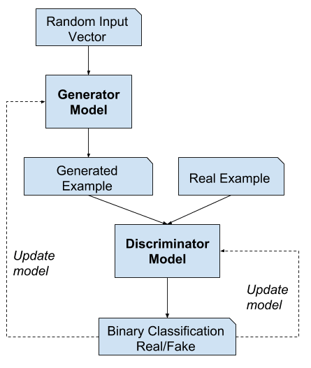
Generative Adversarial Networks(GANs) are a type of deep learning model that is used for generating new data samples which closely look like real data samples. Generally, generative modeling is an unsupervised learning task that tries to discover the regularities or patterns automatically in the input data, and on the basis of that patterns, the model generates new data. But GANs is a super way as a generative model by framing the problem as a supervised learning task with two sub-models. They are:

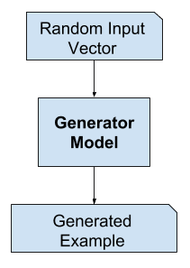
• Generator Model 

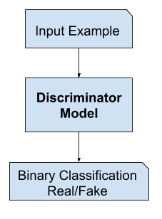
• Discriminator Model

Generator Model

The generator model tries to create new data samples from a random input noise vector called latent space. In GANs, the latent vector serves as input to the generator and represents a point in the latent space that encodes the features of the data. GANs can generate realistic data samples by sampling and transforming different latent vectors. It’s goal to generate new samples that closely look like real data distribution from the problem domain. It tries to create fake samples and tries to look like realistic data by fooling the discriminator. It has no direct access to the input data. The generator model generates the data samples to fool the discriminator.

Discriminator Model

The discriminator model can be called a classifier model. Generally, this model differentiates the real data samples (actual dataset) and fake data samples which are generated by the generator model. The goal of the discriminator model correctly identifies whether the given input is real or fake. 

Applications as well as Types of GANs

Now we have learned about the basic two sub-models (Generator & Discriminator) of GANs. Before deep dive into how GANs work stepwise, it is needed to understand in which sectors we can use this method to increase motivation of learning the GANs properly. There are a lot of applications where GANs are used properly and the number of applications increases day by day as well as a number of variants in the field of GANs for different perspectives. Today we will just look at the names of them and maybe in other articles we will discuss more depth about those variants. They are:

• Vanilla GAN: This is the original GAN that is proposed by Lan Goodfellow. The architectures of generator and discriminator models generally use fully connected layers. Basic image generations, learning the foundation principal of GANs are the applications of it.

• Conditional GAN (CGAN): It is a variant of GANs that add additional conditional information (class labels, attributes or others) to the both generator model and discriminator model. Image generation, data augmentation, style transfer, anomaly detections and others are the applications of CGAN. Here is a paper about it.

• Deep Convolutional GAN (DCGAN): It uses the convolutional layers in both generator and discriminator architectures to make them suitable for image synthesis tasks. Image generation, style transfer, art creation, conditional video generation, data augmentation, image to image translation are the applications of CGAN.

• StarGAN: It is used for multi-domain image-to-image translation. It uses a single generator and discriminator model to learn the mappings/patterns from the multiple domains and performs image translation between any two domains. Style transfer, cross domain image transfer and others are the applications of StarGAN.

• BigGAN: This model is designed for generating high-quality, high-resolution images for large-scale image generation tasks like ImageNet. Large scale and high fidelity image generation  are the applications of BigGAN, producing detailed and realistic virtual environments for gaming, generating unique, high-quality textures for 3D modeling are the applications of BigGAN.

• Laplacian Pyramid GAN (LAPGAN): This model is used to generate high-resolution images with improved visual quality. Hierarchical image generation, visualization of different abstraction levels of images, producing images for varying levels of detail based on the hierarchical model are the applications of LAPGAN.

• Super Resolution GAN (SRGAN): SRGAN is designed for single image super-resolution tasks. The goal of SRGAN is to generate high-resolution images from low-resolution images. Enhancing the resolution of images (image super-resolution), improving video quality by increasing the resolution of frames, enhancing old or low-quality CCTV footage for analysis, refining medical images for improved diagnostics, upgrading old movies or photos to high resolution and others are the applications of SRGAN.

• Wasserstein GAN (WGAN): It is a type variant of GANs that introduce the new training objective based on the wasserstein distance. This new objective is used to mitigate the problems which are faced by traditional GANs. Generating more stable and high-quality images due to stable training dynamics, producing realistic animations and virtual simulations, augmenting data in domains that require high stability, realistic content generation for virtual environments and others are the applications of WGAN.

• CycleGAN: It is used for the unpaired image-to-image translation tasks. It introduces a cycle consistency loss that enforces the consistency between the forward and backward translations that allow the model to learn from two different domain without paired data. Unpaired Image to image translation (examples: horse to zebra, summer to winter scenes and others) can be the applications of CycleGAN, converting types of images, like photos to paintings are the applications of CycleGAN. Unpaired image to image translation (examples: horse to zebra, summer to winter scenes and others), converting types of images, like photos to paintings are the applications of CycleGAN.

• StyleGAN: It is used for controlling the generation process using style and noise inputs. It can produce high-quality, diverse and customizable samples. Generating hyper-realistic human faces, as showcased by sites like 'This Person Does Not Exist', stylized content creation for art and media are the applications of StyleGAN.

These are the few variants of GANs. There are many more variants such as InfoGAN, Pix2Pix, DiscoGAN, SAGAN (Self Attention GAN), 3D GAN, Text to Image GANs(Stack GANs), FUNIT, SinGAN, and so on. The variants of GANs are increasing day by day. 

There are a lot of applications with respect to GANs and day by day, the demand of using GANs is increasing. Hope you feel interested to learn the GAN deeply. Okay. Let’s go deep.

How GANs Works and Generate Plausible New Data

To understand the process of GANs working, It is needed to deeply understand the full meaning of GANs. GANs stands for generative adversarial networks. The three components are generative, adversarial & network.

• Generative: It refers to the process of generating or creating new data samples. This aspect comes from the generator model which is responsible for generating new realistic data samples. The primary goal of a generator model is to learn the underlying data distribution of the training dataset so that it can create plausible new data. It focuses to capture the structure and patterns of the real data and create new realistic data.

• Adversarial: It means the competitive process between two sub-models (generator model and discriminator model). Here, two things happen, The generator tries to generate realistic data samples to fool the discriminator and the discriminator model tries to correctly identify whether a given sample is real data sample or fake. The adversarial training process pushes the generator to create better samples over time so that it can cheat with the discriminator, while the discriminator model becomes more efficient to identify the real or fake data samples. This competition during training time can be called adversarial in GANs.

• Networks: We know that the generator and discriminator models are trained simultaneously in GANs. Now, the architecture of the generator and discriminator model is called the networks. The generator and discriminator model can design in various layers or architectures such as fully connected layers, convolutional layers, recurrent layers, and so on. The architecture of the two sub-models depends on the specific tasks.

We have learned the three main terms of GANs. Overall, the generator model generates new data samples, and then the discriminator checks the samples fake or real. If the discriminator tells that the given sample is fake, then the generator gets feedback in the form of gradients through backpropagation and updates the weights of the network. The continuous process occurs until the discriminator becomes a fool. When the discriminator model becomes fool means it is harder time for the discriminator to identify whether the given sample is real or fake, then the discriminator gives the output of the generated data samples as real at the time of generating realistic data samples by generator. And also the weights of the generator model don’t update when it becomes successful to cheat the discriminator. 

Simply the learning of GANs can be two parts. They are

• The aim of the generator model is to minimize the difference between real and generated samples with the help of getting feedback from the discriminator model. When the Discriminator model identifies the fake data, it gives feedback to the generator to update the weights of the networks to make more plausible data. At the time when discriminator fails to identify the fake data, It might not provide any useful gradients for the generator learn form. 

• The discriminator model tries maximum to distinguish the fake and real data samples. As the generator improves to generate realistic data, the discriminator loses its performance to distinguish the real and generated data samples. This whole process is done by the adversarial networks.

Hope the concept of the GAN is clear. Cool. We have learned the concept and a lot of things about GANs. You can learn more here.  Let’s go into coding Part. 

Hands-on Coding Part

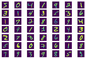
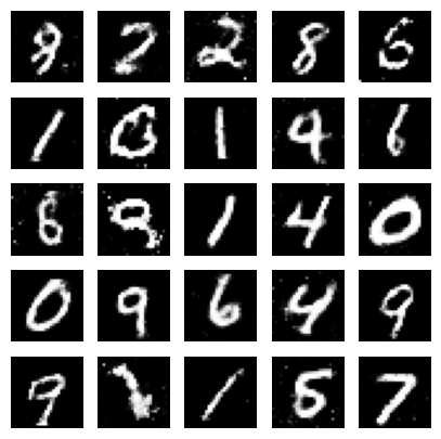
Today we will generate images as like as MNIST dataset. We know that the MNIST dataset contains 70000 images of 10 digits(0 to 9). All the images are in grayscale form. The resolution of each image is 28 *28 pixels. The images look like this.

We will train our discriminator model with the MNIST dataset and will provide some noise same to MNIST to the generator to generate new plausible images that look like a realistic MNIST dataset. Let’s get started. You will get the full code in Google Colab also.

Tensorflow

Import required Libraries

# Import the necessary modules from Keras
from keras.layers import Input, Dense, Reshape, Flatten
from keras.layers import BatchNormalization
from keras.layers import LeakyReLU
from keras.models import Sequential, Model
from keras.optimizers import Adam
# Import matplotlib for plotting
import matplotlib.pyplot as plt
# Import numpy for numerical operations
import numpy as np
# Import the MNIST dataset from TensorFlow Keras
from tensorflow.keras.datasets import mnist

Just imported some associate libraries that will be used to create the generator and discriminator model. MNIST dataset is taken from the keras dataset library. Adam is taken for optimization technique, Leaky Relu for the activation function, and Batch Normalization for the Normalizing technique. Sequential and Model create the model structure.

The MNIST image size is (28*28). Because of a grayscale image, I add the channel number 1. So the overall image shape is (28*28*1).

img_rows = 28
img_cols = 28
channels = 1
img_shape = (img_rows, img_cols, channels)

Generator Model

GANs are based on two sub-models (Generator Model and Discriminator Model). The generator will generate images from noise data. Here, I make a generator model in the build_generator function. Noise_shape is the input latent vector. Then Sequential is called for creating a model. In this model., three fully connected layer is used with 256, 512 & 1024 units.LeakyRelu activation is used to mitigate the vanishing gradient problem.Batch normalization is used to increase training speed and stability. The output of the generator is the same as the training image output (28*28*1) and at last output layer consists of Tanh activation which gives the output [-1 to 1]. Then as input noise_shape (1D array of size 100) is taken and call our generator model in img variable. At last Keras model class is returned connecting the noise as input and img(generated image) as output tensor.

# Function to build the generator model responsible for generating new images.
def build_generator():
    noise_shape = (100,)  # 1D array of size 100 (latent vector / noise)
    # Create a Sequential model representing the generator.
    model = Sequential()
    # Add a fully connected layer with 256 neurons and LeakyReLU activation.
    model.add(Dense(256, input_shape=noise_shape))
    model.add(LeakyReLU(alpha=0.2))
    # Add Batch Normalization to stabilize the learning process and improve convergence.
    model.add(BatchNormalization(momentum=0.8))
    # Add another fully connected layer with 512 neurons and LeakyReLU activation.
    model.add(Dense(512))
    model.add(LeakyReLU(alpha=0.2))
    # Add Batch Normalization to the second layer.
    model.add(BatchNormalization(momentum=0.8))
    # Add another fully connected layer with 1024 neurons and LeakyReLU activation.
    model.add(Dense(1024))
    model.add(LeakyReLU(alpha=0.2))
    # Add Batch Normalization to the third layer.
    model.add(BatchNormalization(momentum=0.8))
    # Add a final fully connected layer with the number of neurons equal to the total number of pixels in the target image.
    # The 'tanh' activation function is used to ensure that the pixel values in the generated image are in the range [-1, 1].
    # This is common for GANs as they use the tanh activation for better stability during training.
    img_shape = (28, 28, 1)  # Image shape for MNIST (28x28x1)
    model.add(Dense(np.prod(img_shape), activation='tanh'))
    # Reshape the output to the target image shape (28x28x1 in this case).
    model.add(Reshape(img_shape))
    # Print the summary of the generator model showing the layers and parameters.
    model.summary()
    # Define an Input layer for the noise input.
    noise = Input(shape=noise_shape)
    # Generate an image using the previously defined model by passing the noise input through it.
    img = model(noise)  # Generated image
    # Return a Keras Model object representing the generator, taking noise as input and generating an image as output.
    return Model(noise, img)

Discriminator Model

build_discriminator  function creates the discriminator model for GANs. Discriminator model is almost as like as binary classification. It will take an image and classify the image as real or fake. The model consists of some layers such as Flatten, Dense layer, and LeakyRelu layers. At first Flatten layer converts the image shape(28*28*1) into a 1D vector (784). Three Dense layers as fully connected layers. The first two dense layers are hidden layers with 512 & 256 units. The last Dense layer is used as Output layer with a sigmoid activation function for binary classification. LeakyRelu with alpha 0.2 is used as an activation function in the hidden layers. At last, I take the img as input with (28*28*1) image shape and validity as output(fake or real) and return the Keras Model Class connecting the input and output.

# Function to build the discriminator model responsible for distinguishing between real and generated images.
def build_discriminator():
    # Create a Sequential model representing the discriminator.
    model = Sequential()
    # Add a Flatten layer to convert the 28x28x1 image into a 1D array.
    img_shape = (28, 28, 1)  # Image shape for MNIST (28x28x1)
    model.add(Flatten(input_shape=img_shape))
    # Add a fully connected layer with 512 neurons and LeakyReLU activation.
    model.add(Dense(512))
    model.add(LeakyReLU(alpha=0.2))
    # Add another fully connected layer with 256 neurons and LeakyReLU activation.
    model.add(Dense(256))
    model.add(LeakyReLU(alpha=0.2))
    # Add a final fully connected layer with 1 neuron and a sigmoid activation function.
    # The output of this layer represents the probability that the input image is real (output is 1) or fake (output is 0).
    model.add(Dense(1, activation='sigmoid'))
    # Print the summary of the discriminator model showing the layers and parameters.
    model.summary()
    # Define an Input layer for the image input (real or generated).
    img = Input(shape=img_shape)
    # Determine the validity of the input image (real or generated) using the previously defined model.
    # The output will be a single value representing the probability of the input image being real (1) or fake (0).
    validity = model(img)
    # Return a Keras Model object representing the discriminator, taking an image as input and producing the validity score as output.
    return Model(img, validity)

Train Function

This function is used to train the GAN model by the training process that involves updating the generator and discriminator model. The function takes three arguments (epochs, batch_size, save_interval). Epochs are the number of training iterations. Batch size is the number of images processed in each iteration. Save_interval means after a number of epochs the model saves the generated images. 

MNIST dataset is taken from the keras mnist dataset. Then Normalize the image into (-1 to 1) and add the channel in the image that becomes (28*28*1). Then define half_batch by taking half of batch_size. Now it is time to iterate the model through random half-batch images in a specific epoch. 

Take random values of 1D vector with half batch size as idx variable. Take the images according to the idx numbers in img variable. Define the noise with (half_batch * 100) size. Now generate the image from noise by generator model. Then detect the loss for real and fake images separately and take the average loss as discriminator loss. 

Now train the generator model. First, take the noise as (batch_size*100) size. Then run the combined model(generator and discriminator combined) with the target set value is one that generator can generate images that look real according to the discriminator. Then compute the generator loss. And after a specific number of epochs save images by the save_imgs function.

# Function to train a Generative Adversarial Network (GAN) using the MNIST dataset.
def train(epochs, batch_size=128, save_interval=50):
    # Load the MNIST dataset and preprocess the data.
    (X_train, _), (_, _) = mnist.load_data()

    # Convert pixel values to floats and rescale them to the range [-1, 1].
    X_train = (X_train.astype(np.float32) - 127.5) / 127.5

    # Add a channel dimension to the images to match the input shape of the generator and discriminator (28x28x1).
    X_train = np.expand_dims(X_train, axis=3)

    # Calculate the batch size for the discriminator (half real, half fake images).
    half_batch = int(batch_size / 2)

    # Training loop: iterate over the specified number of epochs.
    for epoch in range(epochs):
        # ---------------------
        #  Train Discriminator
        # ---------------------

        # Select a random half batch of real images from the dataset.
        idx = np.random.randint(0, X_train.shape[0], half_batch)
        imgs = X_train[idx]

        # Generate random noise as input for the generator.
        noise = np.random.normal(0, 1, (half_batch, 100))

        # Use the generator to create a half batch of fake images.
        gen_imgs = generator.predict(noise)

        # Train the discriminator on real and fake images separately.
        # Research has shown that separate training is more effective.
        # The discriminator is trained to classify real images as 1 and fake images as 0.
        d_loss_real = discriminator.train_on_batch(imgs, np.ones((half_batch, 1)))
        d_loss_fake = discriminator.train_on_batch(gen_imgs, np.zeros((half_batch, 1)))

        # Calculate the average discriminator loss from real and fake images.
        d_loss = 0.5 * np.add(d_loss_real, d_loss_fake)

        # ---------------------
        #  Train Generator
        # ---------------------

        # Generate random noise as input for the generator.
        noise = np.random.normal(0, 1, (batch_size, 100))

        # Labels for the generator's loss function: all ones (1) indicating that the generated images are valid.
        valid_y = np.array([1] * batch_size)

        # Train the combined GAN model (generator) to maximize the discriminator's error.
        # The generator aims to generate images that the discriminator classifies as valid (1).
        g_loss = combined.train_on_batch(noise, valid_y)

        # Print the progress of training at the current epoch.
        print("%d [D loss: %f, acc.: %.2f%%] [G loss: %f]" % (epoch, d_loss[0], 100 * d_loss[1], g_loss))

        # If at the specified save interval, save generated image samples.
        if epoch % save_interval == 0:
            save_imgs(epoch)

Save images

Save_imgs is for saving images after a specific number of epochs in the training time. How many rows and columns of images do you want that is declared by r(row), c(column)? I take a (5*5) grid of generated images. So before generating an image, define the noise. Here the noise is (25*100) size with a normal distribution. Then generate the number of images through the generator model. Then rescale the generated images in (0 to 1). Then create subplots to make a grid of images in a place and save the image into the machine. 

# Function to save generated image samples during the training process.
def save_imgs(epoch):
    # Set the number of rows and columns for arranging the generated image samples.
    r, c = 5, 5

    # Generate random noise as input for the generator to produce r * c image samples.
    noise = np.random.normal(0, 1, (r * c, 100))

    # Use the generator to create image samples from the random noise.
    gen_imgs = generator.predict(noise)

    # Rescale the generated images from the range [-1, 1] to [0, 1] for visualization.
    gen_imgs = 0.5 * gen_imgs + 0.5

    # Create a grid of subplots to display the generated image samples.
    fig, axs = plt.subplots(r, c)

    # Initialize a counter for traversing the generated images.
    cnt = 0

    # Loop through the grid of subplots and display each generated image sample.
    for i in range(r):
        for j in range(c):
            axs[i, j].imshow(gen_imgs[cnt, :, :, 0], cmap='gray')
            axs[i, j].axis('off')
            cnt += 1

    # Save the figure containing the generated image samples to a file.
    # The file name includes the current epoch to track the progress over training iterations.
    fig.savefig("images_/10000mnist__%d.png" % epoch)

    # Close the figure to free up memory.
    plt.close()

Compile the Models

Adam optimizer is used for optimization with a 0.0002 learning rate and the exponential decay rate for the first-moment estimations (beta_1) is 0.05. This value is commonly used in GAN for a good balance in training speed and stability. 

Then discriminator model is compiled that is created before in the build_discriminator function. It is compiled with binary Cross entropy loss function (2 categories fake/real), Adam optimizer, and accuracy as evaluation metrics.

Then generator model is also compiled which is created before in the build_generator function. It is compiled with binary cross entropy loss and Adam optimizer.

# Define and compile the discriminator and generator models, and create the combined GAN model.
# Create an Adam optimizer with a learning rate of 0.0002 and momentum 0.5.
optimizer = Adam(0.0002, 0.5)

# Build the discriminator model using the function 'build_discriminator'.
discriminator = build_discriminator()

# Compile the discriminator with binary cross-entropy loss and the defined optimizer.
# The discriminator aims to distinguish between real and generated images and predicts a binary output (0 or 1).
discriminator.compile(loss='binary_crossentropy', optimizer=optimizer, metrics=['accuracy'])

# Build the generator model using the function 'build_generator'.
generator = build_generator()

# Compile the generator with binary cross-entropy loss and the defined optimizer.
# The generator aims to generate realistic images that the discriminator classifies as real (1).
generator.compile(loss='binary_crossentropy', optimizer=optimizer)

# Define an Input layer for random noise (latent vector) that serves as input to the generator.
z = Input(shape=(100,))

# Generate an image using the generator by passing the random noise as input.
img = generator(z)

# Freeze the discriminator's weights during GAN training.
discriminator.trainable = False

# Define the combined GAN model that links the generator and discriminator.
combined = Model(z, img)

# Compile the combined GAN model with binary cross-entropy loss and the defined optimizer.
# The combined GAN aims to generate images that the discriminator classifies as real (1).
combined.compile(loss='binary_crossentropy', optimizer=optimizer)

Okay. We have compiled the generator and discriminator model. Now we have to combine two modes in a combined model and that needs to compile. Now z is the noise input for the generator, img (generated image)  is the output of the generator function that is the input for the discriminator, and the discriminator gives the output as valid or invalid. So, the combined model connects the input as noise and the output as fake or real. Then compile the combined model with binary cross entropy loss because the output of the combined model is either real or fake and with Adam optimizer. Now our model is ready to train. 

Train The Models 

 I have created a train function before. Now gives the parameter like epochs as 100, batch_size is 32 and save images after 50 epochs(save_interval). And also see the last 5 epochs of the training. 

train(epochs=100, batch_size=32, save_interval=50)
1/1 [==============================] - 0s 50ms/step
95 [D loss: 0.005964, acc.: 100.00%] [G loss: 4.440216]
1/1 [==============================] - 0s 60ms/step
96 [D loss: 0.012839, acc.: 100.00%] [G loss: 4.668732]
1/1 [==============================] - 0s 38ms/step
97 [D loss: 0.020863, acc.: 100.00%] [G loss: 4.605138]
1/1 [==============================] - 0s 54ms/step
98 [D loss: 0.015600, acc.: 100.00%] [G loss: 4.889931]
1/1 [==============================] - 0s 39ms/step
99 [D loss: 0.007563, acc.: 100.00%] [G loss: 4.761877]

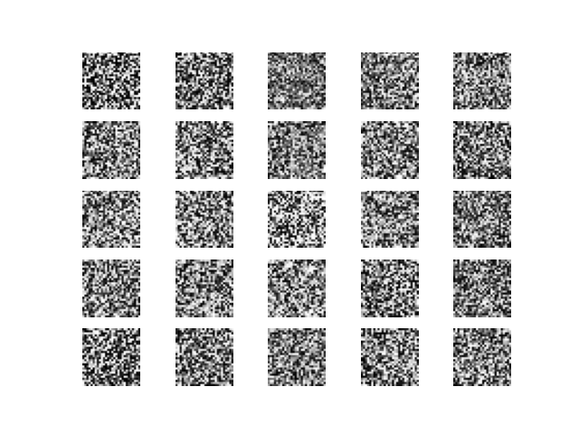
The Generator generates the (5*5) grid images after 100 epochs. Look likes almost same as noise input.

Train with 500 epochs

After training 500 epochs, the generator generates images that are clear than 100 epochs generator. See the last 5 epochs of the model and generated image visualization.

combined = Model(z, valid)
combined.compile(loss='binary_crossentropy', optimizer=optimizer)
train(epochs=500, batch_size=32, save_interval=100)
1/1 [==============================] - 0s 18ms/step
494 [D loss: 0.646408, acc.: 62.50%] [G loss: 0.738816]
1/1 [==============================] - 0s 18ms/step
495 [D loss: 0.664116, acc.: 50.00%] [G loss: 0.736084]
1/1 [==============================] - 0s 24ms/step
496 [D loss: 0.626099, acc.: 62.50%] [G loss: 0.723899]
1/1 [==============================] - 0s 19ms/step
497 [D loss: 0.653843, acc.: 56.25%] [G loss: 0.756174]
1/1 [==============================] - 0s 20ms/step
498 [D loss: 0.639507, acc.: 62.50%] [G loss: 0.755493]
1/1 [==============================] - 0s 18ms/step
499 [D loss: 0.631184, acc.: 71.88%] [G loss: 0.757412]

Okay. Cool. With increasing the number of epochs, the model can generate images much better over time. Now train the model with 5000 epochs. See the output of the last 5 epochs and the visualization of generated images.

combined = Model(z, valid)
combined.compile(loss='binary_crossentropy', optimizer=optimizer)
train(epochs=5000, batch_size=32, save_interval=1000)
1/1 [==============================] - 0s 27ms/step
4994 [D loss: 0.629062, acc.: 62.50%] [G loss: 0.893581]
1/1 [==============================] - 0s 22ms/step
4995 [D loss: 0.617955, acc.: 71.88%] [G loss: 0.870173]
1/1 [==============================] - 0s 24ms/step
4996 [D loss: 0.633161, acc.: 62.50%] [G loss: 0.878531]
1/1 [==============================] - 0s 25ms/step
4997 [D loss: 0.552921, acc.: 71.88%] [G loss: 0.912011]
1/1 [==============================] - 0s 22ms/step
4998 [D loss: 0.673476, acc.: 56.25%] [G loss: 0.842822]
1/1 [==============================] - 0s 22ms/step
4999 [D loss: 0.606060, acc.: 65.62%] [G loss: 0.963637]

The generated images are more clear than before. 

Let’s increase the epochs more and see the output of the last 5 epochs and visualisations of generated images.

combined = Model(z, valid)
combined.compile(loss='binary_crossentropy', optimizer=optimizer)
train(epochs=10000, batch_size=32, save_interval=999)
1/1 [==============================] - 0s 23ms/step
9992 [D loss: 0.641209, acc.: 68.75%] [G loss: 0.835109]
1/1 [==============================] - 0s 22ms/step
9993 [D loss: 0.607246, acc.: 78.12%] [G loss: 0.946683]
1/1 [==============================] - 0s 25ms/step
9994 [D loss: 0.675804, acc.: 56.25%] [G loss: 0.956217]
1/1 [==============================] - 0s 25ms/step
9995 [D loss: 0.576259, acc.: 81.25%] [G loss: 0.939513]
1/1 [==============================] - 0s 25ms/step
9996 [D loss: 0.684361, acc.: 43.75%] [G loss: 0.883493]
1/1 [==============================] - 0s 24ms/step
9997 [D loss: 0.751227, acc.: 43.75%] [G loss: 0.878193]
1/1 [==============================] - 0s 23ms/step
9998 [D loss: 0.718671, acc.: 62.50%] [G loss: 0.895041]
1/1 [==============================] - 0s 25ms/step
9999 [D loss: 0.711221, acc.: 56.25%] [G loss: 0.859410]

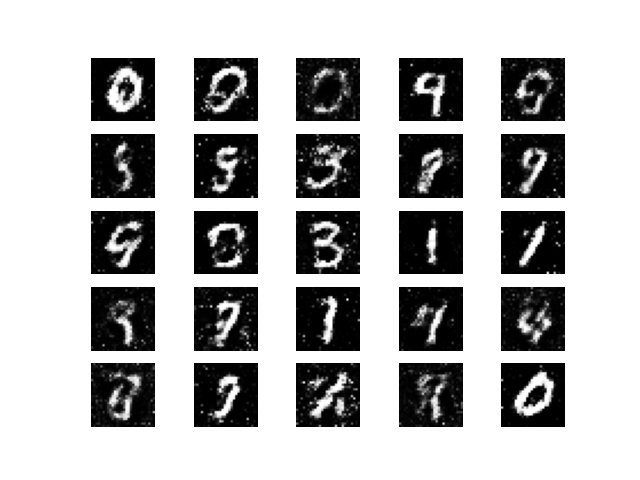
Now The generated images is almost good and realistic to the real images.

Pytorch

Let’s import the necessary libraries to implement the GAN. torch.nn provides the layers, loss functions, and activations functions. Optim module gives the optimization techniques. Torchvision gives MNIST dataset and transforms that is used for data preprocessing, and augmentation. DataLoader effectively loads the data by handling batching, shuffling, and parallel data loading and matplotlib is used for visualization.

import torch
import torch.nn as nn
import torch.optim as optim
from torchvision import datasets, transforms
from torch.utils.data import DataLoader
import matplotlib.pyplot as plt

Generator Model

The generator model is used to generate images in the GAN model. Here the model consists of several fully connected layers with Relu activation functions except for the activation for the output layer. The activation of the output layer is tanh. The input of the generator model is 1D vector of size (100,) and the output is (28*28) size. The fully connected layer units are 256, 512, 1024. 

The forward method defines the forward pass through the network by taking input noise, passing it through the model, and returning the generated output image.

class Generator(nn.Module):
    def __init__(self):
        super(Generator, self).__init__()
        self.model = nn.Sequential(
            nn.Linear(100, 256),
            nn.ReLU(),
            nn.Linear(256, 512),
            nn.ReLU(),
            nn.Linear(512, 1024),
            nn.ReLU(),
            nn.Linear(1024, 28*28),
            nn.Tanh()
        )
    def forward(self, x):
        return self.model(x)

Discriminator Model

The Discriminator model is responsible for classifying the given sample as real or fake. In this discriminator model, some fully connected layers, LeakyRelu, the sigmoid activation function is used. Leaky Relu is used in hidden layers and sigmoid is used in output layers. It takes (28*28) image size as input and gives output real/fake(binary classification). The forward method is doing the same thing as the generator model.

class Discriminator(nn.Module):
    def __init__(self):
        super(Discriminator, self).__init__()
        self.model = nn.Sequential(
            nn.Linear(28*28, 1024),
            nn.LeakyReLU(0.2),
            nn.Linear(1024, 512),
            nn.LeakyReLU(0.2),
            nn.Linear(512, 256),
            nn.LeakyReLU(0.2),
            nn.Linear(256, 1),
            nn.Sigmoid()
        )
    def forward(self, x):
        return self.model(x)

Data Loading and Preprocessing

MNIST Dataset is taken from torchvision datasets module. The transform converts the image data into tensor datatype and normalize with a mean 0.5 and standard deviation of 0.5. Dataloader loads the data effectively with batch size 100, and keeps shuffling true to shuffle the data before each epoch.

transform = transforms.Compose([
    transforms.ToTensor(),
    transforms.Normalize(mean=(0.5,), std=(0.5,))
])
mnist_data = datasets.MNIST(root='./data', train=True, transform=transform, download=True)
data_loader = DataLoader(mnist_data, batch_size=100, shuffle=True)

Noise function 

It will return noise 2D tensors that will be used as generator input. 

def noise(size):
    return torch.randn(size, 100)

Train the Model

Epochs mean the number of iterations of training. Batch_size indicates the size of each batch of images. For the generator and discriminator model, two instances are taken as their name.

The Binary Cross Entropy loss function is taken as a criterion. For the generator model, optimizer_G is taken and for the discriminator model, optimizer_D is taken and both are used Adam optimizer with learning rate=0.0002. 

# Training parameters
epochs = 50
batch_size = 100
# Create generator and discriminator
generator = Generator()
discriminator = Discriminator()
# Loss function and optimizers
criterion = nn.BCELoss()
optimizer_G = optim.Adam(generator.parameters(), lr=0.0002, betas=(0.5, 0.999))
optimizer_D = optim.Adam(discriminator.parameters(), lr=0.0002, betas=(0.5, 0.999))

In each epoch, all the images will be trained. Take the batch of images and reshape the images in 2D tensor(batch_size, 28*28) as real_images. Create real_labels as (batch_size,1). Then compute the discriminator’s output as real_output. Then calculate the BCE Loss. 

Now train the discriminator with fake images. So, Generate noise tensor first as z. Then generate fake images by generator from z. Then create fake labels as (batch_size,1)with zero values. Then compute the discriminator’s output on fake/generated images. Now compute the BCEloss function between fake output & fake labels.  Then sum the two losses as d_loss. Zero out of the gradients of the generator, perform backpropagation, and update the gradient’s parameters. At last print the progress of the model and save the model. 

for epoch in range(epochs):
    for i, (real_images, _) in enumerate(data_loader):
        batch_size = real_images.size(0)
        # Train the discriminator with real images
        real_images = real_images.view(batch_size, -1)
        real_labels = torch.ones(batch_size, 1)
        real_output = discriminator(real_images)
        d_loss_real = criterion(real_output, real_labels)
        # Train the discriminator with fake images
        z = noise(batch_size)
        fake_images = generator(z)
        fake_labels = torch.zeros(batch_size, 1)
        fake_output = discriminator(fake_images.detach())
        d_loss_fake = criterion(fake_output, fake_labels)
        # Update the discriminator
        d_loss = d_loss_real + d_loss_fake
        discriminator.zero_grad()
        d_loss.backward()
        optimizer_D.step()
       
        # Train the generator
        fake_output = discriminator(fake_images)
        g_loss = criterion(fake_output, real_labels)
        # Update the generator
        generator.zero_grad()
        g_loss.backward()
        optimizer_G.step()
    # Print out the progress
    print(f"Epoch: {epoch+1}/{epochs}, d_loss: {d_loss.item()}, g_loss: {g_loss.item()}")
# Save the trained generator
torch.save(generator.state_dict(), "mnist_generator.pth")

The Output of the last few epochs is given below. 

Epoch: 44/50, d_loss: 0.95421302318573, g_loss: 1.4430636167526245
Epoch: 45/50, d_loss: 1.0638306140899658, g_loss: 0.9523686170578003
Epoch: 46/50, d_loss: 1.008470058441162, g_loss: 1.3438955545425415
Epoch: 47/50, d_loss: 0.9164902567863464, g_loss: 1.9861092567443848
Epoch: 48/50, d_loss: 0.8828264474868774, g_loss: 1.3192412853240967
Epoch: 49/50, d_loss: 1.0978505611419678, g_loss: 0.9635183811187744
Epoch: 50/50, d_loss: 0.8551716804504395, g_loss: 1.574243426322937

Generate Image using trained model and Visualize

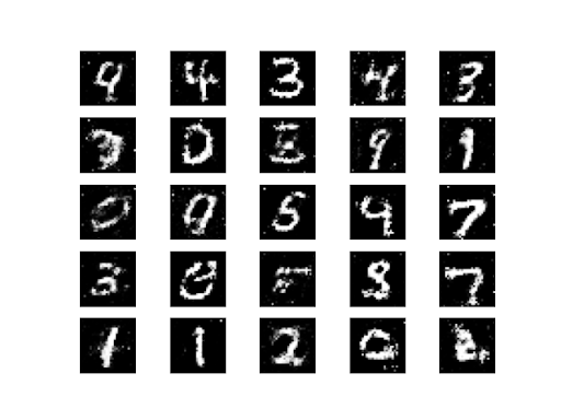
Our model is already trained. Now we will generate new images with our generator model. At first, at the evaluation process, Disables gradient calculation by torch.no_grad(). Now generate noise for 25 samples. Then generate the images through the generator model. At last, The generated images are displayed through subplots in a 5*5 grid of images.

# Visualize generated images
generator.eval()
with torch.no_grad():
    z = noise(25)
    generated_images = generator(z).view(-1, 1, 28, 28).detach().cpu()
fig, axs = plt.subplots(5, 5, figsize=(5, 5))
for i, ax in enumerate(axs.flatten()):
    ax.imshow(generated_images[i, 0], cmap='gray')
    ax.axis('off')
plt.show()

The generated images look like when the Epochs is 50. The generated images are almost realistic. 

Great. We have learned how to solve a GAN problem in hands-on coding. The Output of the model is quite Good. Let’s Know about some frequently asked questions about GAN to build the Basic more clear.

Frequently Asked Questions About GANs

GANs become very popular because of their highly efficient generating power. Beginner practitioners face a lot of questions about GANs, Now I am going to discuss some of them that can come into the mind while learning GANs so depth. Let’s start.

What is the role of the Generator model and Discriminator model in GANs?

The generator model tries to generate new plausible data samples that look like training data and the Discriminator model tries to identify whether the given input samples are fake or real. With the help of a generator and discriminator model simultaneously, GAN can generate a new realistic dataset.

What is a minimax-2 player game and how it is related to GAN?

In this game, two players take turns making moves, and the outcome of the game depends on the sequence of moves taken by the players. Here, each player tries to make the best moves according to opponent's strategy and like that opponents do the same. In GAN, the generator model generates the new sample and tries to fool the discriminator and the discriminator tries best to identify the sample as fake or real. With the collaboration of each other, the training process goes forward. So, it is related to the minimax-2 player game.

What is DualGAN? Give a brief application of it.

It is a variant of GAN architecture that is designed for image-to-image translation. It has the ability to translate images between two domains using unpaired training data. It can be used in Style transfer, Domain Adaptation, Data Augmentation, Video to video translation, and so on.

What is the difference between Variational Autoencoder and GAN?

Both two are generative models & discriminators, but the processes of them are different. GANs are trained through Adversarial Process, and VAE is trained through Optimization Process. GANs can generate more realistic data samples than VAE. GAN is used in a wide range of distributions while VAE is used limited range of distribution. VAE is easy to train while GAN is a little bit complex to train. Those are the main difference between them.

Which variants of GANs are used to text to image generation?

There are several variants of GANs which can generate plausible images based on a given text description. Among them, I just put some of them such as Conditional GAN(CGAN), Text to Image GAN(T2l-GAN), StackGAN, AttnGAN, MirrorGAN, and so on.

Which kinds of GANs can be used as feature Learning?

Almost all kinds of GANs can be used for feature learning, just need to take the discriminator model for downstream tasks and also need to avoid the generator part of GANs. Some GANs can be used like DCGAN, Auxiliary Classifier GAN(AC GAN), Self Attention GAN and so on.

Why Deep Convolution GAN(DCGAN) is better than Vanilla GAN?

DCGANs are used with convolutional layers while Vanilla GANs is used with fully connected layers. So, DCGANs can learn the complex patterns of the input data where Vanilla GANs can’t. DCGAN is more stable and generates high-quality samples over Vanilla or traditional GAN.

Which variants of GANs are used to solve the stability problem during the training phase?

To address the stability issues of traditional GAN. Some variants of GAN can be used in this perspective such as Wasserstein GAN(WGAN), WGAN-GP, SN-GAN, LSGAN, SAGAN, and so on.

To upgrade the resolution of GANs, which types of GANs can be used?

Some GANs have been designed to enhance the resolution of images such as Super Resolution GAN (SRGAN), Enhanced Super Resolution GAN(ESRGAN), SPLE-GAN, and so on.

Which GANs are responsible to generate a large amount of data samples?

There are some GANs in this perspective like BigGANs, StyleGAN and Style GAN2, ProGAN, and others.

How GANs can be used in Medical Image Synthesis?

It can be used in various perspectives in Medical images. I am giving some of them like to get a large amount of data, GAN can be used in Data Augmentation, GAN can be helpful to solve the imbalance dataset, It can be helpful for privacy preservation and much more cause exist.

Why GANs are so popular today?

There are several causes of become popular. I am giving some causes such as High-quality data Generation, Improved architectures day by day and professionalism in specific tasks, impressive results in unsupervised and semi-supervised learning, power of dealing real-world applications, research interest, and so on.

Can GAN be used as a Data Augmentation technique?

Sure. GAN generate new data that looks like realistic data samples and those can be used in training deep learning model or can deal with other problem. For generating more realistic data, GAN is a very powerful technique. 

The above questions are common questions with respect to GAN. In this article, we have learned the whole concept of GAN, Applications of GANs, Types of GANs, How to code in Tensorflow or Pytorch and visualize the output, and at last learn some extra question that gives more knowledge about GAN. Overall, we have learned a lot of things that are very interesting and fascinating.