Long Short Term Memory(LSTM) Networks | Deep Learning

Long Short-Term Memory, also referred to as LSTM in artificial neural networks, is a potent and sophisticated architecture created to overcome the limitations of conventional recurrent neural networks (RNNs). RNNs are excellent at handling sequential data, making them essential in various applications like time series forecasting, speech recognition, and natural language processing. It is designed to handle the vanishing gradient problem in traditional RNNs. The vanishing gradient problem occurs when the gradient signal becomes very small during the backpropagation algorithm, which can cause the network's weights not to be updated effectively.

How LSTM Differs from RNN

Traditional RNNs suffer from the vanishing gradient problem, which occurs when the gradient signal becomes very small during the backpropagation algorithm, making it difficult to update the network's weights effectively. It is particularly problematic when the network needs to remember information from many steps back in the sequence, such as in natural language processing tasks or speech recognition.

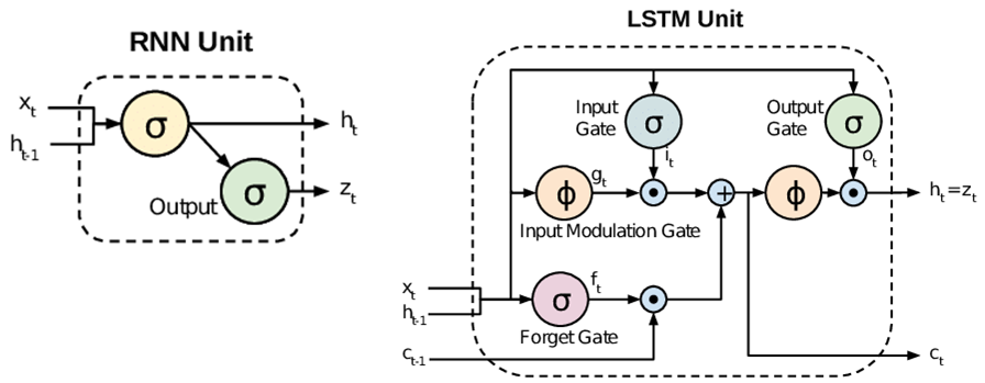
LSTM networks address this issue by introducing a memory cell that can selectively remember or forget information over long periods, allowing the network to handle long-term dependencies in sequential data effectively. By using the three gates (input, fail, and output) in the LSTM cell, the network can selectively update its memory and control the flow of information, resulting in improved performance on tasks that require modeling long-term dependencies.

Architecture of LSTM

LSTM (Long Short-Term Memory) is a recurrent neural network (RNN) type for vanishing gradient problems that can occur with traditional RNNs. LSTMs are particularly effective at modeling long-term dependencies in sequential data, such as natural language text or speech.

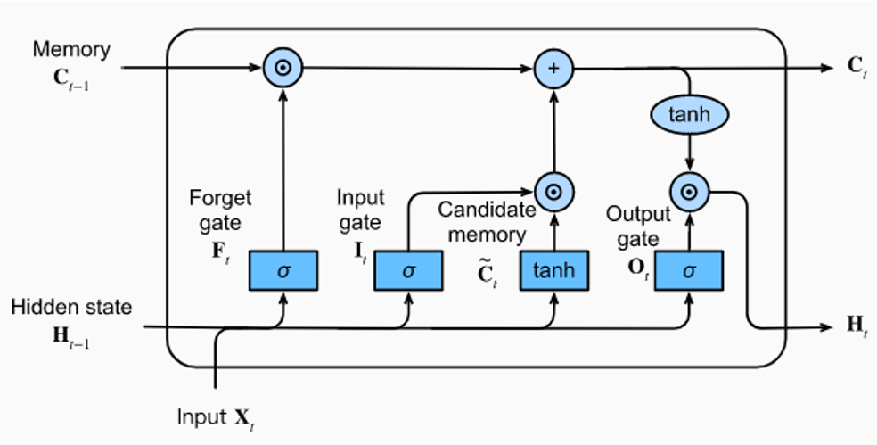
The architecture of an LSTM cell has four main parts: 

• Memory Cell: It's an essential LSTM memory. Its cell is the main LSTM cell. It can store sequence data liable for keeping the long-term memory of the network. It also writes and erases information from its memory over time.
• Input Gate: The input gate is the first gate with a sigmoid function layer that controls which information from the input and the previous hidden state should be in the memory cell.
• Output Gate: The output gate is another sigmoid layer that controls which information from the memory cell should be output as the final hidden state.

In addition to the above three components, LSTMs have a forget gate, another sigmoid layer that controls which information in the memory cell should be overlooked or deleted. The forget gate prevents the LSTM from storing irrelevant or outdated information.

The LSTM architecture is piled to make a deep LSTM network, where multiple LSTM layers are stacked individually various. The result from each LSTM layer is used for input to the next LSTM layer, and the last LSTM layer produces the final outcome of the deep LSTM network.

The LSTM architecture allows the network to selectively save and regain data from the long-term memory while bypassing the vanishing gradient problem that can occur in traditional RNNs. LSTMs are a robust tool for modeling sequential data with long-term reliance.

Anatomy of an LSTM cell 

LSTM cell applies a chain of memory blocks to four connected neural network architectures. The standard LSTM unit comprises a cell, an input gate, a forget gate, and an output gate. These gates regulate the flow of data into and out of the cell and permit the cell to have dealt with over an extended duration. LSTMs are specially fitted to take me a series of data of differing sizes, making them sufficient for categorizing, interpreting, and expecting such data. You will get the full code in Google Colab also.

Implementation of LSTM in Tensorflow

# Import necessary libraries
# Import the 'drive' module from Google Colab to mount Google Drive and access data
from google.colab import drive
# Mount Google Drive to access files and folders stored on Google Drive
# The user will be prompted to authenticate and provide access to their Google Drive
drive.mount('/content/drive')
# Import NumPy library for numerical operations and array manipulations
import numpy as np
# Import Pandas library for data manipulation and analysis
import pandas as pd
# Import MinMaxScaler from scikit-learn to scale data to a specific range
from sklearn.preprocessing import MinMaxScaler
# Import TensorFlow library, a popular deep learning framework, for building and training models
import tensorflow as tf
# Import the 'Sequential' class from Keras to build a sequential neural network model
from keras.models import Sequential
# Import the 'LSTM' and 'Dense' layers from Keras to construct the neural network architecture
from keras.layers import LSTM, Dense
# Import the 'pyplot' module from Matplotlib to create visualizations
import matplotlib.pyplot as plt
# Import 'mean_squared_error' function from scikit-learn to evaluate model performance
from sklearn.metrics import mean_squared_error

from math import sqrt

# Dataset you can download here
# Read the data from the CSV file in Google Drive
df = pd.read_csv('/content/drive/MyDrive/AAPL.csv')

# Scale the 'Close' data using Min-Max scaling to bring values between 0 and 1
scaler = MinMaxScaler(feature_range=(0, 1))
scaled_data = scaler.fit_transform(df['Close'].values.reshape(-1, 1))

# Split the data into training and test sets
training_size = int(len(scaled_data) * 0.8)
test_size = len(scaled_data) - training_size
train_data = scaled_data[0:training_size, :]
test_data = scaled_data[training_size:len(scaled_data), :]

# Define a function to create sequences from the data for input and output
def create_sequences(data, seq_length):
    X, y = [], []
    for i in range(len(data) - seq_length - 1):
        X.append(data[i:(i + seq_length), 0])  # Input sequence
        y.append(data[i + seq_length, 0])      # Output value for the sequence
    return np.array(X), np.array(y)

# Set the sequence length for the LSTM model
seq_length = 60

# Create input-output sequences for training and testing data
X_train, y_train = create_sequences(train_data, seq_length)
X_test, y_test = create_sequences(test_data, seq_length)

# Reshape the input data to fit the LSTM model
X_train = np.reshape(X_train, (X_train.shape + (1, )))
X_test = np.reshape(X_test, (X_test.shape + (1, )))

# Define the LSTM model using Keras Sequential API
model = Sequential()
model.add(LSTM(50, return_sequences=True, input_shape=(seq_length, 1)))  # LSTM layer with 50 units
model.add(LSTM(50))  # Another LSTM layer with 50 units
model.add(Dense(1))  # Dense output layer with 1 unit

# Compile the model using Adam optimizer and mean squared error loss function
model.compile(optimizer='adam', loss='mean_squared_error', run_eagerly=True)

# Train the LSTM model using the training data
model.fit(X_train, y_train, epochs=10, batch_size=32)

# Evaluate the model on training and test data
train_predict = model.predict(X_train)
test_predict = model.predict(X_test)

# Inverse transform the scaled data to original scale
train_predict = scaler.inverse_transform(train_predict)
y_train = scaler.inverse_transform([y_train])
test_predict = scaler.inverse_transform(test_predict)
y_test = scaler.inverse_transform([y_test])

# Calculate and print the Root Mean Squared Error (RMSE) for training and test data
train_score = np.sqrt(mean_squared_error(y_train[0], train_predict[:, 0]))
test_score = np.sqrt(mean_squared_error(y_test[0], test_predict[:, 0]))
print('Train Score: {:.2f} RMSE'.format(train_score))
print('Test Score: {:.2f} RMSE'.format(test_score))

# Make predictions on the test data
predictions = model.predict(X_test)

# Inverse transform the scaled predictions to original scale
predictions = scaler.inverse_transform(predictions)

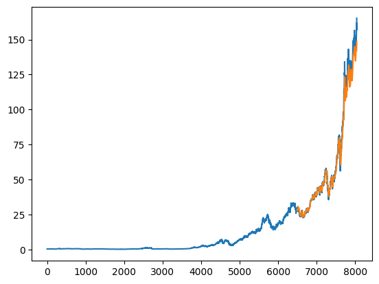
# Plot the original 'Close' values and the predicted values for the test set
plt.plot(df['Close'].values)  # Original 'Close' values

plt.plot(range(training_size + seq_length + 1, len(df['Close'])), predictions)  # Predicted values
plt.show()

Applications of LSTM

LSTM networks have used sequential modeling for a wide range of time series data applications, specifically those that need modeling long-term dependencies. There are some real-world examples of the use of LSTM networks:

• Language modeling: when we write anything on Google or youtube, we see that some common words are suggestions for us; LSTM networks for creating language modeling tasks, where the goal is to predict the probability of a sequence of words given a context. LSTM networks have shown significant improvements over traditional n-gram models and have been used in applications such as speech recognition, machine translation, and text prediction.
• Speech recognition: LSTM networks have speech recognition tasks, which aim to transcribe spoken words into text. LSTM networks have significantly improved over traditional hidden Markov models (HMMs) and have in commercial speech recognition systems such as Siri and Google Voice.
• Music generation: LSTM networks have music generation tasks, where the goal is to generate new music based on a given musical style or genre. It will be changing music in industry LSTM networks trained on large music datasets and used to create music indistinguishable from human-composed music.
• Video analysis: LSTM networks have been used in video analysis tasks, such as action recognition and video captioning. LSTM networks are used to recognize human actions in videos and to generate descriptive captions that describe the content of the video. It can change video graphics and advertisement marketing. 
• Stock market prediction: LSTM networks are used in stock market prediction tasks, where the goal is to predict the prospective expense of a stock based on chronological data. LSTM networks have been used to model the convoluted worldly connections in economic data and have shown profitable outcomes in forecasting stock prices.

Advanced LSTM Techniques

Let's look at a real example where LSTM was used to forecast stock prices. A-LSTM has been demonstrated to be efficient for a number of applications, including time series forecasting, emotion recognition, and natural language processing. A-LSTM outperformed the traditional LSTM by 5.5% in research on emotion recognition. On the GLUE benchmark, A-LSTM produced cutting-edge results in a study on natural language processing. Additionally, in time series forecasting research, A-LSTM outperformed the traditional LSTM in accuracy across various datasets. You can learn more about A-LSTM from here 

The following are some benefits of A-LSTM over traditional LSTM:

• It is more efficient at capturing long-term dependencies.
• It is more robust to noise.
• It is easier to train.

 In general, LSTM has one hidden layer, but in advanced, have multiple layers. There has someone: 

• Stacked LSTM: The stacked LSTM is an extension of this model with numerous hidden LSTM layers, including various memory cells. The stacked LSTM hidden layers make the model deeper, more accurately earning the description as a deep learning technique. The depth of neural networks is attributed to the approach's success on various challenging prediction problems.
• Bidirectional LSTM: A Bidirectional LSTM (biLSTM) is a sequence processing model that consists of two LSTMs: one carrying the input in a forward trend and the other in a backward trend. BiLSTMs effectively improve the knowledge known to the network, improving the context open to the algorithm and learning what words directly follow and forego a comment in a penalty.
• LSTM with attention mechanism: In this situation, we need to give more weight to it. Basic LSTM requires clarification between the terms and, occasionally, can envision the wrong word.

Conclusion

In the article, we have learned about the Long Short-Time Memory(LSTM) network, its use cases, and implemented an LSTM network in TensorFlow. LSTM has been a revolutionary technology in deep learning research and development and using LSTM we can solve a lot of real-world problems.