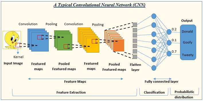
Convolutional Neural Networks | Deep Learning

A convolutional neural network(CNN) is a type of deep learning algorithm that has capable to learn the hierarchical features from the data automatically. Think of CNNs as a special computer program that can recognize things in pictures. Just like how we can tell apart a cat from a dog by looking, CNNs help computers do the same. They're like the computer's eyes! They are widely used to extract features from the data and becomes popular in computer vision, NLP related tasks.

CNN is widely used in a lot of real-life applications in the area of deep learning. Including:

• Image classification
• Object detection
• Instance / Semantic segmentation 
• Optical character recognition
• Image style transfer
• Medical image analysis
• Autonomous vehicles and so on.

How CNN Model Works

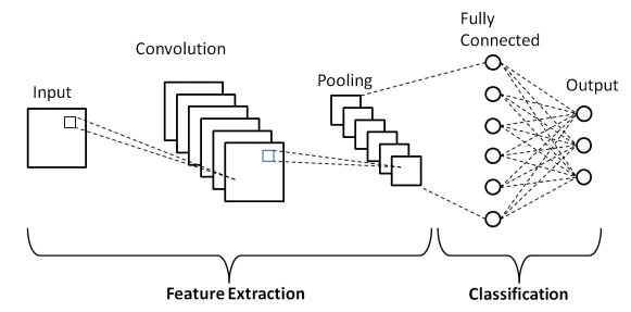
A CNN model consists of some layers such as convolutional layers, activation functions, pooling layers, fully connected layers, and output layers. Let’s know the concept of each layers step by step.

• Convolutional Layers: It performs convolutional operations on the data using a set of filters. Each filter tries to detect the features from the data. It is designed to automatically and adaptively learn spatial hierarchies of features from input images or sequences.

• Activation Function: After completing the convolutional operations, the output features of the convolutional layers are goes to the activation function to introduce the non-linearity into the network so that the network can learn complex patterns and representations from the data. Generally ‘relu’ activation function is used in the hidden layers. 

• Pooling Layers: It reduces the spatial dimensions that are generated by convolutional layers. It helps to decrease the number of parameters of the model and reduce the complexity and computational power. Some pooling methods are max pooling, average pooling, global max pooling, and global average pooling.

• Fully Connected Layers: After convolutional layers and pooling layers, one or more fully connected layers are used to aggregate the learned features and help to make accurate predictions.

• Output Layers: It is the final layer of the CNN model that produce the prediction or classification of the input data. For binary classification, Sigmoid activation is used and for multiclass classification, SoftMax activation is used.

These are the basic layers in convolutional neural networks. There may be other layers such as the dropout layer, normalization layers, and so on.

Types of CNN

There are different types of CNN based on Various tasks. Including:

• 1D CNN: Here the CNN kernel moves in one direction, generally used in time series data.

• 2D CNN: Here the CNN kernel moves in two directions (up & down). Generally used in computer vision related tasks.

• 3D CNN: Here the CNN kernel moves in three direction(up, down & inside). Generally used in 3D images like CT Scans, MRIs, etc.

Let’s understand CNN in depth with an example.

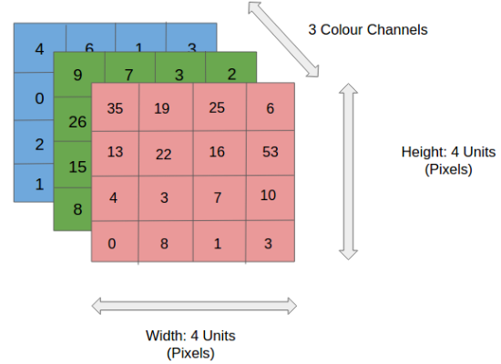
Suppose we have an image in RGB format means it has 3 channels. Image is nothing but a matrix. If the image is in grayscale format, the channel will be 1. Now take a look at RGB image below

Convolutional Layers

To apply convolution operation on the image, we have to tell the filters, kernel size, strides, padding, kernel initializer, and other hyperparameters. 

• A filter is a number that determines how many features the layer can learn from the data.

• Kernel Size specifies the height & width of the convolutional kernel. It is a small matrix that slides across the input data during convolution operation. The kernel matrix can be (3,3) or (5,5) or any custom matrix. The matrix is learnable parameter during backpropagation and helps the model to accurately classify. Larger kernel like (9,9) matrix or more captures the large features of the image where small kernel captures small features.

• Strides specify the number of steps for the kernel as it moves across the input data, both horizontally and vertically. A larger stride value makes smaller feature maps and a smaller stride value makes larger feature maps.

• Kernel Initializer initializes the kernel weights. It indicates the defining the value of the kernel matrix before training so that the model can update the kernel matrix properly during backpropagation. There are some popular initializers such as ‘he normal’, ‘locan_uniform’,’glorot_uniform’, and so on. Proper kernel initialization can be helpful to remove the vanishing or exploding gradient problems in the neural network.

• The padding determines the strategy for handling borders. The two main operations of padding are:

             1.  ‘Same’ padding pads the input data so that the output feature maps have the same dimension as the input data. It adds zero value in the border of the input before performing convolutional operations and keeps same dimensions in the output features as input data.

             2. ‘Valid’ padding doesn’t add any pads in the input data. So the output feature maps become smaller than the input data.

There are also other hyperparameters that exist to perform a CNN model. Above discussion for convolutional layers. Now, In a RGB image, the convolution operation visualization is given below

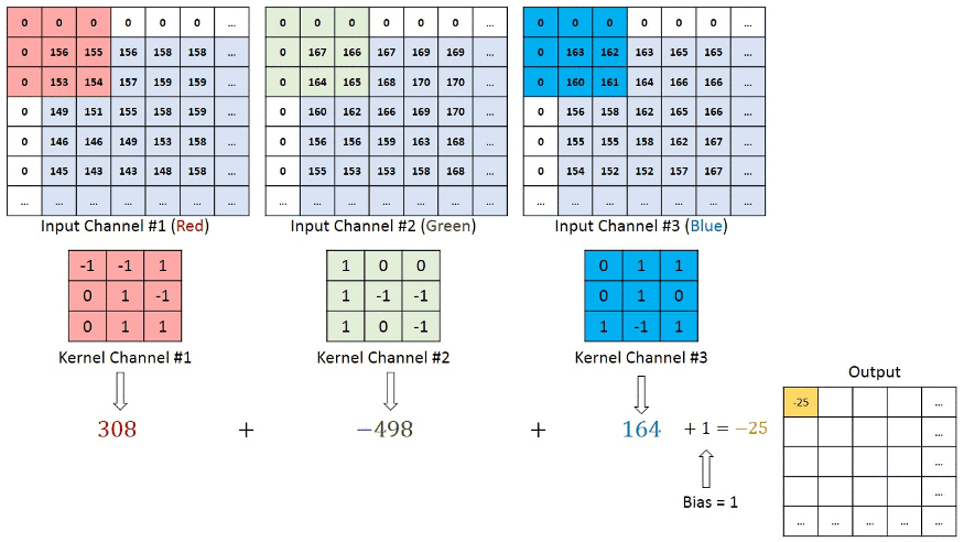
Here kernel_size is a (3,3) matrix that is moving one step right and after then one step below means (1,1) strides with same padding (zero including border to keep same dimensions of output features as input to perform the convolution operation. After performing convolutional operation, the output stores the value in the output features and feed those as input into another layer.

Operation of Pooling Layers

After the convolution operation, pooling methods come into place. Pooling layers are used in feature maps that come from convolution layers to reduce the spatial dimensions. Pooling layers help the model to reduce the dimension and complexity of the model. So, the model becomes fast.

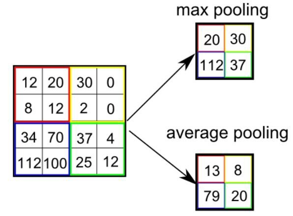
The pooling operation is performed with a specified window size and stride over feature maps. The window size is a (2*2) or (3*3) matrix and stride determines how many step sizes for moving the window across the feature maps. There are some pooling operations such as max pooling, average pooling, global max pooling, and global average pooling. 

• Max pooling takes the maximum value within each region that is selected as the output of the region.

• Average pooling takes the average value within each region that is selected as the output of the region

Generally pooling operation works by applying aggregated function(max, average) to non-overlapping regions of the input features and also reducing the dimension of the output features. 

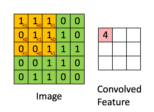
Look to have a good idea about pooling. Here, a (3*3) window moves (1*1) strides and takes the maximum values as the output feature.

In the below image, here the window size is (2*2) and the strides is (2*2). So, the window moves 2 steps and for max pooling it takes the maximum value in each window and for average pooling, the output features take the average value.

So the overall architecture for the CNN model is 

INPUT  —-> CONVOLUTION LAYERS —> POOLING LAYERS —> FULLY CONNECTED LAYERS —> OUTPUT

Okay. Hope you can understand the concept of how a CNN model works. Now let’s solve a image classification problem by the CNN model and see the performance by predicting the unseen data. 

Tensorflow

Let’s start by importing the required packages. You will get the full code in Google Colab also.

import numpy as np
import tensorflow as tf
from tensorflow.keras import layers, models
from tensorflow.keras.datasets import mnist
from tensorflow.keras.utils import to_categorical
import matplotlib.pyplot as plt

Our image classification performs on MNIST data that consists of 70000 images where 60000 images are for training and 10000 images for Testing the model. Each image size is 28*28 pixels. I take the MNIST data from the Keras dataset library. ‘To_categorical’ is used for one hot encoding of the labels of images and ‘matplotlib’ library for visualization.

Load The Data & Visualize images

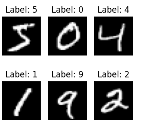
At first, I load the images and labels and also split the data into the training part and testing part. Then visualize the first 6 images from the training images and has shown the labels also. You can see different images by changing the value of image indices. Then create a subplot to show all the images in a place. The code looks like

(train_images, train_labels), (test_images, test_labels) = mnist.load_data()
# Choose the indices of the images 
image_indices = [0, 1, 2, 3, 4, 5]
# Create a 2x3 grid for displaying 6 
imagesfig, axes = plt.subplots(2, 3, figsize=(3, 3))

for i, ax in enumerate(axes.flat): 
    ax.imshow(train_images[image_indices[i]], cmap='gray') 
    ax.set_title(f"Label: {train_labels[image_indices[i]]}") 
    ax.axis('off')
    plt.tight_layout()
    plt.show()

See the images of the first 6 from training images and labels also

Data Preprocessing

It is a very necessary step before modeling the data. According to Keras API, our MNIST data is split into training parts and testing parts. One more part is Validation data that is used in the training time to check whether the model can learn perfectly or not. So, take some data as validation data from training data.

from sklearn.model_selection import train_test_split
# split the images and labels for training and testing
X_train, X_val, y_train, y_val = train_test_split(train_images, train_labels, test_size=0.2, random_state=23)
print(X_train.shape, X_val.shape, test_images.shape)

Output:

(48000, 28, 28) (12000, 28, 28) (10000, 28, 28)

So, the number of training images is 48000, vvalidation images are 12000 and testing image is 10000 and each image size is 28*28 pixels. Now, format each image into 28*28*1 pixels in grayscale format. The last 1 is the channel number. After reshaping training images, validation images, and testing images, normalizing all the images by dividing 255 so that the value of all images becomes 0 to 1.  Then I convert the labels into one hot encoding for all training labels, testing labels & validation labels.

# add one channel in the last for grayscale image

X_train = X_train.reshape((48000, 28, 28, 1))

# normalize the image fixels into (0 to 1)
X_train = X_train.astype('float32') / 255
X_val = X_val.reshape((12000,28,28,1))
X_val = X_val.astype('float32') /255
test_images = test_images.reshape((10000, 28, 28, 1))
test_images = test_images.astype('float32') / 255

# convert the labels into one hot encoding
y_train = to_categorical(y_train)
y_val = to_categorical(y_val)
test_labels = to_categorical(test_labels)

Model Creation

Three times, I took 2D Convolutional layers where filters are 32,64 & 64 and strides are (3*3) and Relu activation function. A 2D Maxpooling is taken with (2*2) window size. A Flatten layer is used to convert the feature maps into a 1D vector. Then A fully Connected layer is used with 64 units and Relu activation function. Finally, the output layer with 10 units because the image has 10 categories and softmax activation for multiclass classification.

# create model

model = models.Sequential()

# convolutional layers with (3,3) kernel and produce 32 features 
model.add(layers.Conv2D(32, (3, 3), activation='relu', strides=(1,1),padding='valid', kernel_initializer='glorot_uniform', input_shape=(28, 28, 1)))

# Max pooling layer with (2,2) window size

model.add(layers.MaxPooling2D((2, 2)))
model.add(layers.Conv2D(64, (3, 3), activation='relu'))
model.add(layers.MaxPooling2D((2, 2)))
model.add(layers.Conv2D(64, (3, 3), activation='relu'))

# convert the 2 dimensional features into 1 dimensional features
model.add(layers.Flatten())

# fully connected layers with 64 neurons

model.add(layers.Dense(64, activation='relu'))

# output layer with 10 neurons for 10 labels 
model.add(layers.Dense(10, activation='softmax'))

Compile & Train the Model

Adam is used as an optimizer that is widely used in image classification tasks because of its faster convergence and better performance. The loss function is categorical crossentropy that is commonly used for multiclass classification. It calculates the cross-entropy loss between one hot encoded true labels and the predicted probabilities output of the model. Accuracy metrics evaluate the performance of the model during training.

model.compile(optimizer='adam', loss='categorical_crossentropy', metrics=['accuracy'])

The model is ready to run. I take (X_train, y_train) as training data, (X_val,y_val) as validation data for measuring the performance of the model during training. Epochs 20 means the model iterated 20 times and the batch size has taken 64 which indicates entire dataset will be divided into 64 batches and one batch will be runinng in each iteration.

history = model.fit(X_train,y_train, epochs=20,validation_data = (X_val,y_val), batch_size=64)

Epoch 15/20750/750 [=====================] - 3s 5ms/step - loss: 0.0067 - accuracy: 0.9977 - val_loss: 0.0414 - val_accuracy: 0.9912
Epoch 16/20750/750 [=====================] - 3s 4ms/step - loss: 0.0059 - accuracy: 0.9982 - val_loss: 0.0517 - val_accuracy: 0.9903
Epoch 17/20750/750 [=====================] - 4s 5ms/step - loss: 0.0078 - accuracy: 0.9976 - val_loss: 0.0466 - val_accuracy: 0.9899
Epoch 18/20750/750 [====================] - 4s 5ms/step - loss: 0.0037 - accuracy: 0.9987 - val_loss: 0.0571 - val_accuracy: 0.9899
Epoch 19/20750/750 [=====================] - 5s 6ms/step - loss: 0.0056 - accuracy: 0.9981 - val_loss: 0.0796 - val_accuracy: 0.9864
Epoch 20/20750/750 [=====================] - 4s 5ms/step - loss: 0.0045 - accuracy: 0.9984 - val_loss: 0.0466 - val_accuracy: 0.9913

Now let’s see how our model can perform in unseen data(test Image). I evaluate the model with a test image and got 99% accuracy. That’s awesome. 

test_loss, test_acc = model.evaluate(test_images, test_labels)
print(f'Test accuracy: {test_acc}')

Test accuracy: 0.9926000237464905

Prediction & Visualize

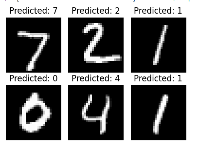
Now I took the first 6 images and predict those images through our model and get the predicted labels. Then visualize those images with their predicted labels in a 2*3 grid of subplots. Let’s see the code below.

# Choose the indices of the images you want to predict
image_indices = [0, 1, 2, 3, 4, 5]
# Create a 2x3 grid for displaying 6 images and their predictions
fig, axes = plt.subplots(2, 3, figsize=(4, 3))
for i, ax in enumerate(axes.flat):
    input_image = test_images[image_indices[i]].reshape(1, 28, 28, 1) 
    prediction = model.predict(input_image) 
    predicted_class = np.argmax(prediction)
    ax.imshow(test_images[image_indices[i]].reshape(28, 28), cmap='gray') 
    ax.set_title(f"Predicted: {predicted_class}") 
    ax.axis('off')
plt.tight_layout()
plt.show()

The visualization looks like this where the first six test images are given and their predicted labels are also given.

Frequently Asked Questions & Answers on CNN

CNN is a widely used deep learning model, especially for computer Vision. So, many practitioners face many problems in terms of using CNN. Now I will discuss some problems and answers at a time. Let’s get started.

What are the advantages of using CNN over ANN?

It can detect important features of complex data (image, audio, video, or raw data) automatically and no need for human intervention which is not possible by ANN. Also CNN gives higher accuracy in computer vision tasks over ANN.

What are the techniques to visualize and interpret the features learned by CNN?

There are a few techniques to visualize the feature maps that are learned by convolutional layers such as Saliency Maps, Grad CAM, Deep Dream, and so on.

Why Batch Normalization is used in CNN?

Batch Normalization helps to stabilize and accelerate the training and is useful to mitigate the vanishing or exploding gradient problems by normalizing the inputs of the layers.

What are the advantages of using padding in CNN?

Padding can help to prevent information loss at edges, preserve the spatial dimensions and improve the network’s ability to learn features in the boundaries.

To prevent overfitting in CNN, Which step can be taken?

Some techniques can be taken such as DropOut, Data Augmentation, Regularization Techniques, and so on. If the dataset is small, then data augmentation can be helpful. If network architecture is so complex, then DropOut can be used. Regularization can be used as a practice to reduce overfitting. 

Could you give me some popular CNN Architectures?

Yes. There are many CNN Architectures such as AlexNet, VGG Variants, Resnet Variants, Inception, Xception, and So on.

How CNN can be used in Natural Language Processing(NLP) tasks?

CNN is good at computer vision problems. Although it can solve some NLP problems also like text classification, named entity recognition, relation extraction, semantic role labeling, machine translation, and so on.

How does CNN perform Dimensionality reduction in the network?

After convolutional layers, sometimes pooling layers are used in CNN to perform dimensionality reduction and make the network faster. There are most common pooling layers are MaxPooling, average pooling, and so on.

Overall, we have learned a lot of things about convolution neural networks (CNN). Hope you enjoy the article and idea behind CNN is now fully clear. Thanks.