Optimization Algorithms for Deep Learning | Deep Learning

Optimization is a crucial part of deep learning that is used to update the parameters(weights and bias) of a neural network model in order to minimize the error/loss between the predicted output and the actual output. The goal of an optimizer is to find the set of parameters that minimizes the objective function of the model. 

We should understand the training steps of neural networks. The steps are:

• Forward pass from input data layer to output layer.

• Obtain output and measure the loss between predicted output and actual outputs of the data.

• Backward pass to obtain the gradients and update the network parameters to minimize the loss between predicted output and actual output.

The last step is called the optimization process. In a nutshell, optimizers are used to minimize the loss function by updating the model parameters through a backward pass (backpropagation). Today we will highly discuss the optimization process, algorithms, and associate concepts that are related to optimization techniques. First look at the overview of the tutorials. The tutorials are divided into some parts. Including:

• Introduction 

• Overview of objective function

• Gradient descent algorithms

• Improvements to optimization algorithms

• Comparison of optimization algorithms 

• Practical consideration of optimization algorithms

• Challenges

• Conclusion

Let’s start and build a high knowledge about the core concept(Optimization) in deep learning.

Introduction

Optimization helps to find the best set of parameters for a given model for minimizing the loss function by measuring the difference between the model’s prediction and true labels. By reducing the loss function, the model becomes more accurate in its predictions. The benefits of using the optimization technique are given below.

• Convergence: Optimization algorithms are used to find the set of parameters (weights & biases in the neural networks) that minimize the loss between prediction and actual labels. Convergence to a local or global minimum is important for the model to predict well on unseen data.

• Upgrade training speed: A good optimization algorithm can significantly upgrade the speed of the training process where fast convergence or training process can reduce the time and computational resources also. 

• Adaptability: Some optimization technique has the ability to set the learning rate(hyperparameter) automatically during training. This helps the model to fast convergence to find the optimal solution.

• Robustness: Some optimization algorithms are more robust to noise and other issues and also perform well to generalize unseen data.

• Ease of use: Optimization algorithms are easy to use and implement. 

Overall, optimization algorithms impact the performance, convergence speed, and generalization ability of a deep learning model. This is the core concept of deep learning neural networks.

Types of Optimization Algorithms

There are several types of optimization algorithms that have been developed over time. Now see the names of them and later in the articles can learn the details of the algorithms. They are:

• Gradient descent 

• Stochastic gradient descent

• Mini batch gradient descent

• Gradient descent with momentum

• Nesterov accelerated gradient (NAG)

• AdaGrad

• Adadelta

• RMSProp

• Adam

• Newton’s method

The optimization algorithms are developing over time through researchers. There are many other algorithms such as AdamW, Nadam, AMSGrad, Quickprop, Resilient Propagation(RProp), Hessian free optimization, and so on. Maybe in future articles, we can discuss those optimization algorithms. Today we will discuss the only pointed above optimizer algorithms. One thing, I want to tell you about is that generally optimization algorithm is used as the perspective of the problem. But most of the deep learning practitioners use adam optimizer because of its features. We will learn those step by step in the following articles. 

Overview of Objective Functions

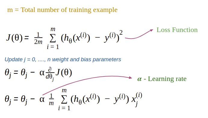
The goal of an optimization algorithm is to minimize the value of the objective function for improving the performance of the model. Here objective function(cost function or loss function) is a mathematical function that measures how well is able to make predictions on unseen data. Different optimization algorithms use different ways to minimize the loss function. Gradient descent and its variants calculate the gradient of the loss function(objective function) with respect to the model parameters(weights, biases) and update the parameters in the direction of the local or global minimum. The second order optimization methods(Newton method) use the second derivative of the objective function to compute the optimal step size for the gradient update. The objective function plays an important fact in the optimization process because the optimization process is computed based on the objective function. The choice of the loss function depends on the specific problem such as regression, classification, or generation. Let’s know some common objective functions in different use cases are given below.

• Mean Squared Error(MSE) Loss: This function is used in regression problem where it calculates the squared differences between the predicted and true values and averages them over all instances. 

• Cross Entropy Loss: This function is used in classification problems by measuring the dissimilarity between the predicted probability distribution and the true distribution. For binary classification, Binary cross entropy loss is used and for multi-class classification, Categorical cross entropy is used.

• Huber Loss: This function is used for regression problem that is less sensitive to outliers and also It combines the best properties of Mean Squared Error and Mean Absolute Error.

• Kullback-Leibler (KL) divergence Loss: It computes the difference between one probability distribution to another. Generally, it is used in the Variational Autoencoder model and other generative models.

• Dice Loss: Generally this function is used in segmentation tasks by measuring the overlap between the predicted and ground truth segmentations. 

Actually, there are many other loss functions such as HInge Loss, Mean Absolute Error(MAE), Log-Cosh Loss, Focal Loss, Cosine Similarity loss, Contrastive loss, Triplet loss, center loss, and so on. Actually, the number of loss functions is increasing day by day. 

Gradient Descent Algorithms

Gradient Descent Algorithms is a type of optimization algorithm that is used to minimize the objective function in Deep learning models. The main idea behind gradient descent is to iteratively update the model parameters in the direction of the steepest descent of the cost function. In other words, This algorithm iteratively updates the parameters of the model in the direction of the negative gradient of the objective function with respect to the model parameters. 

Generally Deep Learning model consists of a lot of parameters that is being updated at the time of the training process by minimizing the chosen loss function. The gradient descent algorithm is an efficient way to find a set of parameters(weights and biases) that minimize the loss function. 

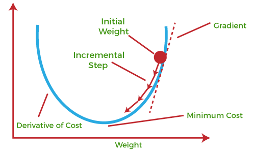
First, the neural network starts with an initial guess for the model parameters. Then calculates the gradient of the loss function with respect to the model parameters. The update of the parameters in the opposite direction of the gradient and the size of the update is determined by the learning rate parameter. This learning rate controls the step size towards the local or global minima and a very important hyperparameter that is needed to tune to get the optimal convergence. 

The algorithms iterate continuously until the loss function converges to the local or global minimum. So the overall process of the gradient descent algorithm is to measure the loss function, compute the gradients of the loss function with respect to the model parameters, update the parameters and the process will iteratively run until the algorithm can converge the loss function to the local or global minima. Now we will learn the definition of some words that are used in this article.

Convex and Non-convex function

Convex is a function where only one minimum point is situated that is called the global minima. There is no local minimum situated. Gradient Descent is guaranteed to converge the global minimum of the loss function if the function is convex and the learning rate is appropriately chosen.

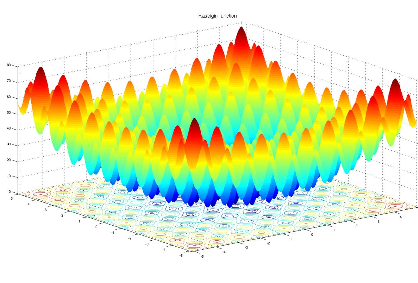
A non-convex function is a function where you can notice the presence of the local minima, global minima, saddle points, and flat regions. Gradient Descent may stuck to converge the global minima of the loss function in the Non-COnvex function. 

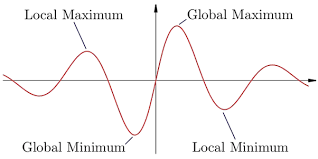
Local Minima, Global Minima & Saddle Points

Local Minima indicates a point that is low compared to its neighboring points but not the lowest point to all the points. Sometimes optimization algorithms identify the local minima as global minima at the time of working non-convex function.

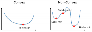
Global Minima is the lowest point of all the points of a function. This means it is the overall minimum value. The goal of any optimization technique is to reach this global minimum point.

Saddle points are the critical points in the landscape when the gradient is zero but the point is neither a local minima nor a global minima. In the non-convex function, there may be a number of saddle points. The problem is the algorithm may be stuck in these points and making no progress.

Learning rate, Learning rate schedule, Weight Decay & Momentum

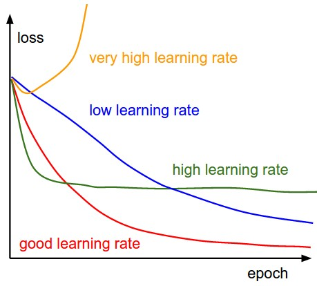
The learning rate determines the step size of the algorithm and controls how much the model parameters are updated in response to the calculated gradient during optimization. A smaller learning rate needs more iterations to converge to the global or local minima when a larger learning rate may lead to faster convergence but can cause the model to overshoot the optimal solution.

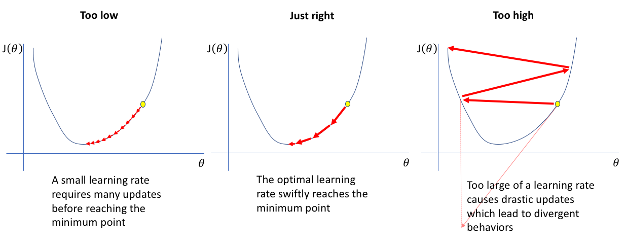
So Choosing an optimal learning rate is very essential to converge the function to the minimum points. Various methods can be used to choose the appropriate learning rate such as Grid Search, Learning rate schedules, Adaptive learning rate, One-cycle policy, and so on. Look at the graph to understand the importance of the appropriate learning rate.

A learning rate schedule is used to decrease the learning rate over time. The idea behind the learning rate schedule is to initialize with a relatively large learning rate and gradually reduce the learning rates as the training progresses. Some common learning rate schedules are Step decay, Exponential decay, Cosine annealing, One-cycle policy, Reduce on the plateau, and so on.

Weight Decay is a regularization technique that is used in optimizers to prevent overfitting by adding a penalty term to the objective function based on the magnitude of the model weights. This penalty encourages the model to have smaller weights which are implemented by multiplying the model weights by a small factor during each update step.

Momentum is used in the optimizer to move quickly in the direction of the optimum by adding a fraction of the previous weight update to the current weight update. In other words, it is used to improve the convergence speed and stability of the gradient-based optimization algorithms.

Cool. you have achieved the basic of Optimization algorithms. Now let’s go forward and gain a deep understanding of the context of optimization algorithms. 

Types of Gradient Descent Algorithm

We know that Gradient Descent Algorithm is used to update the model parameters iteratively during the training process. The variants of the Gradient Descent algorithms depend on the size of the dataset used in every step to update the model parameter. There are mainly three variants of Gradient Descent. They are Batch, Stochastic & Mini-batch Gradient Descent. Let’s go through the deeper discussion of each variant of Gradient Descent.

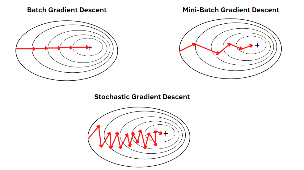
• Batch Gradient Descent: This algorithm updates the model parameters by computing the gradient of the entire dataset at each step. Simply it takes all the datasets in each iteration of the training process and the overall step of Gradient descent is the same. It has advantages and disadvantages too. This algorithm is guaranteed to converge to the minimum of the objective function. But it can be hugely expensive to use especially for large dataset because this method takes all the training examples in each iteration and update the model parameters. And also it may converge slowly to the optimal minima points of the objective function.

• Stochastic Gradient Descent (SGD): This is another type variant of Gradient Descent that updates the model parameters by computing the gradient of only one randomly selected data. To overcome the computational expensiveness, this process has developed. This process introduces noise in the optimization process. It is faster than Batch Gradient Descent but it may overshoot the optimal solution. It is computationally efficient but finding the global minima is tough in this process. Although by appropriate learning rate, it can be possible to reach the global minima by SGD and also it is widely used as a variant of Gradient Descent nowadays. 

• Mini-Batch Gradient Descent: This algorithm is a variant of Gradient Descent that updates the model parameters by computing the gradient of a small subset of the training dataset(mini-batches). It uses a batch of training examples in each iteration that is smaller than all datasets and larger than one data. So, it combines the advantage of Batch Gradient Descent as well as Stochastic Gradient Descent. It is computationally efficient because of taking a small set of data examples and it does not overshoot like SGD. Overall, the mini-batch gradient descent algorithm is more computationally expensive and faster than batch gradient descent and provides smoother convergence and less noise in the weight updates compared to SGD. Simply, it offers a trade-off between Batch Gradient Descent and Stochastic Gradient Descent and a widely used optimization algorithm.

Well. Hope You have gained a lot of knowledge about the Optimization technique and an optimization algorithm namely the Gradient Descent algorithm and its variants. Let’s Discuss the limitations of Gradient Descent.

Limitations of Gradient Descent and its Variants

• In High dimensional non-convex space, This algorithm can stuck in local minima or saddle points and lead to suboptimal solutions not optimal.

• Choosing an appropriate learning rate manually is sensitive. Too large a learning rate can overshoot the optimal solution and too small a learning rate can slowly converge to the optimal solution. 

• The same learning rate is used in all the parameters in every iteration which introduce the lack of adaptability problem.

• The gradients of the loss function can be noisy.

• Vanishing & Exploding problems(details are given below)  can occur in the training process.

There can be issue other problems as well. So, to overcome the problems of Gradient Descent and its variants, many improved optimization algorithms have been developed. We will discuss them now. Stay with us.

Improvements to Optimization Algorithms

To solve the issues of an optimizer, an improved optimizer algorithm had been developed. Now we will discuss some of them such as Gradient Descent with Momentum, Nesterov Accelerated Gradient (NAG), AdaGrad, Adadelta, RMSProp, Adam, Adamax, Newton’s Method, Conjugate Gradient step by step. Let’s start with the topics.

Stochastic Gradient Descent (SGD) with Momentum

Stochastic gradient descent plays noise in the gradients means it provides a zigzag optimization path and potentially converges to an optimal solution slowly. It leads to a high variance in the update direction and may stuck in saddle points and local minima. To overcome that problem, SGD with momentum has developed.

SGD with momentum is a simple addition of momentum in the classic SGD algorithm. SGD with momentum is a method that helps accelerate gradient vectors in the right directions and leads to faster converging. It is a very popular optimization algorithm that works better and faster than SGD.

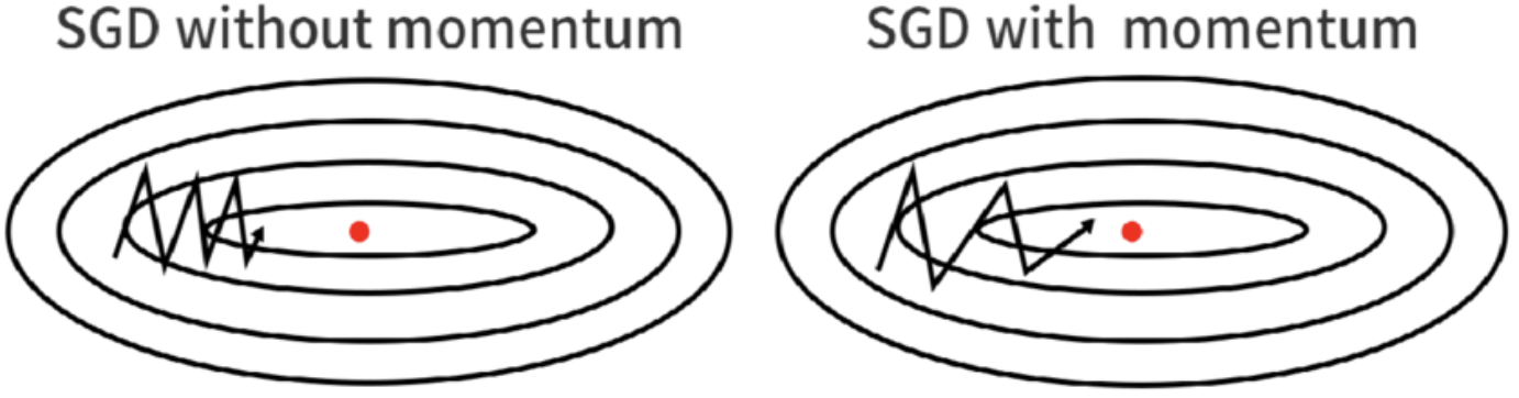
This algorithm can be useful when the data are noisy and the gradients are sparse. It can help to prevent from getting stuck in local minima and saddle points. It can easily traverse in the large non-convex curvature. 

Here, The algorithm keeps track of an exponential moving average of the gradient over time which is called momentum. The momentum helps to smooth out the noise that is defined by the stochastic gradient estimations and helps the optimization process to converge faster to the global minima. 

Here Vdw is the momentum and beta is the momentum hyperparameter. If the beta becomes zero, then the algorithm will convert into gradient descent. 

Overall, SGD with momentum is a variant of SGD that uses an exponentially weighted average of the gradient over time to smooth out the noise and has the ability to converge faster and reach better optima than plain SGD at the time of gradients are noisy or the loss function are highly non-convex.

Nesterov Accelerated Gradient (NAG)

This algorithm is a variant of SGD with momentum. It helps to improve the convergence speed and performance of SGD with momentum and becomes a popular optimization algorithm in Deep learning. The key difference between NAG and SGD with momentum is NAG uses a ‘lookahead’ gradient to update the momentum term rather than the current gradient. This step can lead to more efficient updates of the model parameters.

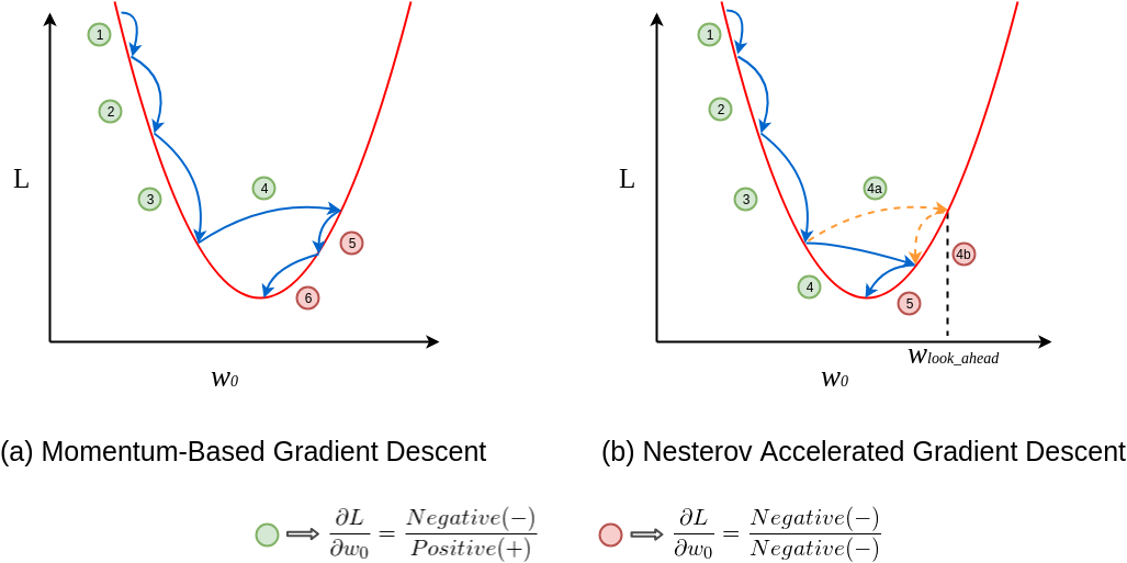
The NAG algorithm updates the model parameters in two steps. Including

• By taking a step in the direction of the current momentum (weighted average of the previous gradient), the model computes the ‘lookahead’ position of the parameters.

• Then it computes the gradient of the cost function at the lookahead position, and using that gradient the model updates the momentum and the model parameters.

The look-ahead step of the algorithm can avoid the overshooting of the cost function and improve convergence speed and accuracy. This optimization algorithm is particularly good for neural networks with many layers and the cost function is highly non-linear. 

Overall, NAG can converge faster and reach better minimum points in the time of noisy gradients and high curvature loss function compare to SGD with momentum. One thing is to notice that it takes additional computation to compute the lookahead step which increases the computational cost of the algorithm. 

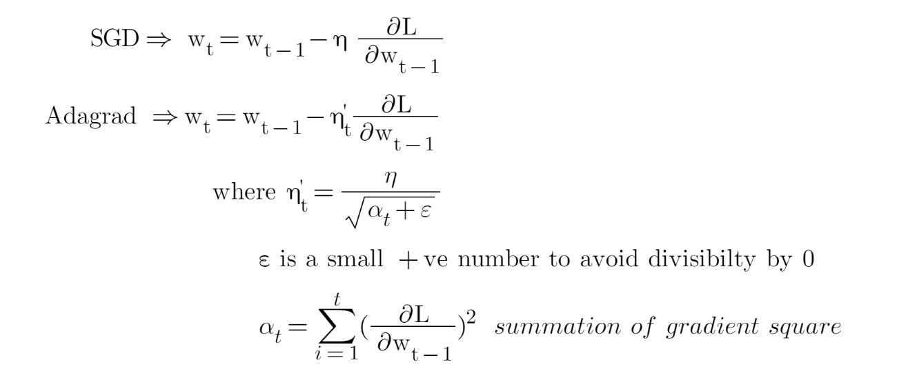
Adaptive Gradient Descent (AdaGrad)

AdaGrad is a gradient-based optimization algorithm that is designed to adaptively adjust the learning rate for each parameter based on the historical gradient information. 

The advantages of using this algorithm are:

• The learning rate is adaptively adjusted for each parameter based on the historical gradient information. 

• Parameters with small gradients will have a larger learning rate which allows the algorithm to converge faster.

• No manual tuning is required.

AdaGrad scales the learning rate for each parameter based on the sum of the squares of the historical gradients. The main idea is parameters with large gradients will have small learning rates and parameters with small gradients will have large learning rates. This makes the algorithms converge faster on parameters.

It has some limitations also which are given below

• Because of accumulating the square gradients over time, the learning rate can be too small which leads to slow convergence and getting stuck in the sub-optimal solutions. 

• It needs high memory for storing the squared gradients for each parameter.

• It may not perform well with noisy or sparse gradients.

Overall, AdaGrad is a type of Optimization Algorithm which can adaptively adjust the learning rate for each parameter based on historical Gradients. Actually, this method provides a feature (adapt the learning rate) as well as some limitations that will be solved by other optimizer algorithms. Let’s go forward.

RMSProp

Root Mean Square propagation(RMSProp) is an optimization algorithm that is developed by Geoff Hinton. In the AdaGrad algorithm, the learning rates are always decreasing and the algorithm does not forget about the past gradients. So, for a long-running task, the learning rate becomes too small. 

To overcome this issue, The RMSprop uses a moving average of squared gradients to normalize the gradients at each iteration. Easily, it uses a moving average of squared gradients at each time step, then divides the gradient by the square root of this average to obtain a normalized gradient. 

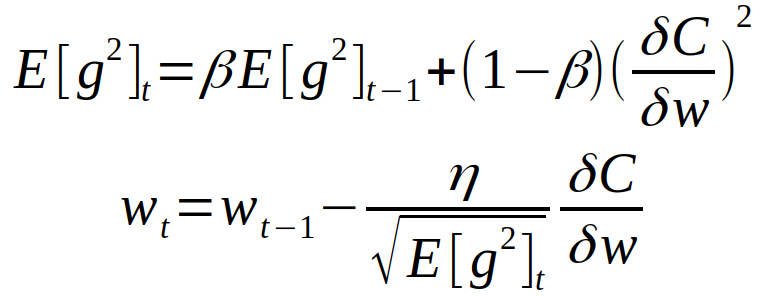
So, the RMSProp resolves the AdaGrad diminishing problem by using an exponential moving average to discard history from the extreme past so that it can converge rapidly. The RMSProp adjusts the learning rate for each weight in the model individually, making it possible to find the global minimum of the loss functions more efficiently. It can work well with sparse gradient and non-stationary objectives and effectively deals with vanishing or exploding gradient problems. 

The RMSProp takes the learning rate and decay rate(additional) as the hyperparameter that is hard to tune. The RMSProp can converge well but not well like more advanced optimizer algorithms(Adam). 

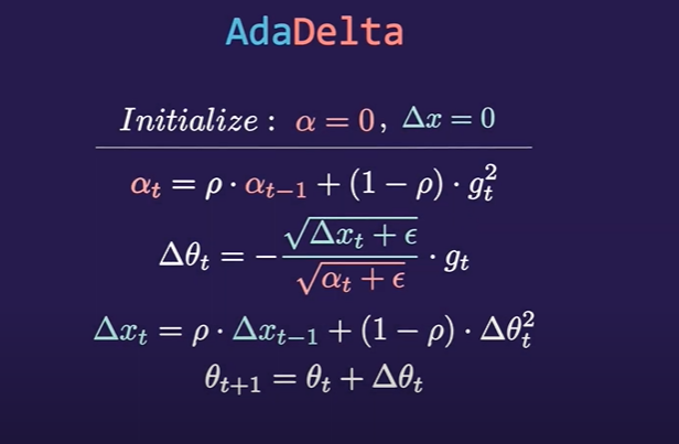
AdaDelta

AdaDelta is an extension of the AdaGrad Optimization algorithm. The AdaGrad optimizer adapts the learning rate for each parameter based on the historical gradient information But It may lead to a very small learning rate(diminishing learning rate problem) over time. To solve the issue of AdaGrad, AdaDelta has been developed. AdaDelta is also called the extension of the RMSProp algorithm.

To overcome the issue of AdaGrad, AdaDelta computes the running average of the gradients and updates to adapt the learning rate instead of the sum of all the squared historical gradients. By replacing the sum of all the squared gradients with a running average of the gradients, the algorithms give better scaling of the learning rate in different parts of the optimization landscape. Adadelta uses a ‘sliding window’ of gradients rather than accumulating all the past gradients. It restricts the window of the past gradients to a fixed size, 

AdaDelta has developed to overcome two problems. Including 

• AdaGrad keeps the learning rate decreasing over time and the learning rate becomes too slower as training progresses. Adadelta has been developed to overcome this problem.

• The need to select a good initial learning rate is hard. Adadelta has come to overcome this problem. In Adadelta, It doesn’t require an initial learning rate setting. 

AdaDelta and RMSProp both use a moving window of past gradients but AdaDelta also keeps track of the accumulation of the parameter updates. AdaDelta restricts this accumulation to a fixed size to a fixed-size window which solves the diminishing learning rate problem.  Adadelta can be more computationally expensive than other optimizer algorithms. 

Adam

Adaptive moment estimation( Adam) is a very popular optimization algorithm that is first introduced in 2014 in a paper named ‘Adam: A method for stochastic Optimization’. It combines the advantages of two popular optimization algorithms are RMSProp and Stochastic Gradient Descent with momentum.

RMSProp adjusts the Adagrad method in a very simple way in an attempt to reduce its aggressive, monotonically decreasing learning rate. It uses a moving average of squared gradients to normalize the gradient itself, which means the learning rate gets adapted over time based on the recent magnitudes of the gradients. 

On the other hand, Momentum optimization helps accelerate the convergence of gradient descent in relevant directions and dampens oscillations. It takes into account the past gradients to smooth out the update.

 Adam was designed to combine these two methods into one algorithm, aiming to leverage their individual strengths while avoiding their weaknesses. Adam computes adaptive learning rates for different parameters. It also calculates an exponentially decaying average of past gradients and squared gradients, and stores these to be used in subsequent gradient steps.

Advantages & Disadvantages

Adam (Adaptive Moment Estimation) is a popular optimization algorithm in deep learning due to its robustness and low requirement for tuning. The advantages of the Adam optimizer are given below. 

• Efficient computation: Adam only requires first-order gradients and the computation requirements for the algorithm are constant in memory, making it suitable for problems with large data or many parameters.

• Applicable to non-stationary objectives: Adam can handle objectives that change over time, making them useful for noisy or online learning problems.

• Robust to noisy/sparse gradients: This feature makes Adam good for datasets with a lot of noise or for sparse data.

• Less sensitive to hyperparameters: Adam doesn’t require much tuning to work well, unlike some other optimization algorithms. The default hyperparameters (learning rate of 0.001, beta1 of 0.9, beta2 of 0.999, and epsilon of 10^-8) often work well.

It has some limitations also that are given below.

• Convergence issue: It's been observed in certain cases that Adam can fail to converge to the optimal solution. This is mainly because the adaptive learning rate could become very small, effectively leading to an early stop of learning.

• Generalization: Some research has shown that models trained using Adam can generalize worse on some datasets compared to those trained with stochastic gradient descent (SGD) and its variants.

• Bias correction problem: Although Adam includes a bias correction mechanism, the estimates of the first and second moment vectors can be biased towards zero, especially during the initial steps, and when the decay rates are small.

Adam optimizer can be applied to various problems in deep learning including Image Recognition, Natural Language Process problems like text classification, sentiment analysis, machine translation, text generation and so on, Generative Adversarial Networks(GANs), Autoencoders, Regression problems, Reinforcement Learning and many more. 

Overall, while Adam is a versatile and powerful optimizer, it isn't always the best choice for every problem. Depending on the specifics of your task and your data, other optimizers may give better results. Always consider experimenting with different optimizers when designing your deep learning models.

Comparison of Optimization Algorithms

We have discussed the concept and advantages, and disadvantages of the optimizer algorithms. We will see the comparison in image classification. Here, We are taking the CIFER-10 dataset and CNN model that will be trained on 5 different optimizers. After completing the train of the model for all optimizers, we will notice which optimizer performs best and which is very bad. You will get the full code in Google Colab also.

import tensorflow as tf
from tensorflow.keras.datasets import cifar10
from tensorflow.keras.utils import to_categorical
from tensorflow.keras.models import Sequential
from tensorflow.keras.layers import Conv2D, MaxPooling2D, Flatten, Dense, Dropout
from tensorflow.keras.optimizers import Adam, RMSprop, SGD, Adadelta, Adagrad

# Load the CIFAR-10 dataset
(x_train, y_train), (x_test, y_test) = cifar10.load_data()
# Normalize the images
x_train = x_train.astype('float32') / 255
x_test = x_test.astype('float32') / 255
# One-hot encode the labels
y_train = to_categorical(y_train, num_classes=10)
y_test = to_categorical(y_test, num_classes=10)

# Define the model architecture
def create_model():
    model = Sequential([
        Conv2D(32, (3, 3), activation='relu', padding='same', input_shape=(32, 32, 3)),
        Conv2D(32, (3, 3), activation='relu', padding='same'),
        MaxPooling2D(pool_size=(2, 2)),
        Dropout(0.25),
        Conv2D(64, (3, 3), activation='relu', padding='same'),
        Conv2D(64, (3, 3), activation='relu', padding='same'),
        MaxPooling2D(pool_size=(2, 2)),
        Dropout(0.25),
        Flatten(),
        Dense(512, activation='relu'),
        Dropout(0.5),
        Dense(10, activation='softmax'),
    ])
    return model

# List of optimizers to compare
optimizers = {
    'Adam': Adam(),
    'RMSprop': RMSprop(),
    'SGD': SGD(),
    'Adadelta': Adadelta(),
    'Adagrad': Adagrad(),
    'Nesterov': SGD(nesterov=True, momentum=0.9)
}

# Train and evaluate the model with each optimizer
histories = {}
for name, optimizer in optimizers.items():
    print(f'Training with {name} optimizer...')
    model = create_model()
    model.compile(optimizer=optimizer, loss='categorical_crossentropy', metrics=['accuracy'])
    history = model.fit(x_train, y_train, batch_size=64, epochs=10, validation_data=(x_test, y_test), verbose=2)
    histories[name] = history

Here, I am just showing the last epoch for all optimizers. Here the best performer is Adam Optimizer because the training and validation loss is lowest than others and the accuracy is most. Adadelta performs very badly here. Anyway, for this experiment, we can’t tell that Adadelta is bad for all experiments. Actually, Deep Learning is a fact of Experiments. More experiments will reach you good results. 

Training with Adam optimizer…
Epoch 10/10
782/782 - 6s - loss: 0.5498 - accuracy: 0.8061 - val_loss: 0.6201 - val_accuracy: 0.7876 - 6s/epoch - 8ms/step
Training with RMSprop optimizer…
Epoch 10/10
782/782 - 6s - loss: 0.6400 - accuracy: 0.7869 - val_loss: 0.8588 - val_accuracy: 0.7561 - 6s/epoch - 8ms/step
Training with SGD optimizer…
Epoch 10/10
782/782 - 6s - loss: 1.2977 - accuracy: 0.5333 - val_loss: 1.2181 - val_accuracy: 0.5669 - 6s/epoch - 7ms/step
Training with Adadelta optimizer...
Epoch 10/10
782/782 - 6s - loss: 2.2422 - accuracy: 0.1623 - val_loss: 2.2280 - val_accuracy: 0.2177 - 6s/epoch - 8ms/step
Training with Adagrad optimizer…
Epoch 10/10
782/782 - 6s - loss: 1.6857 - accuracy: 0.3915 - val_loss: 1.6044 - val_accuracy: 0.4297 - 6s/epoch - 8ms/step
Training with Nesterov optimizer…
Epoch 10/10
782/782 - 6s - loss: 0.6146 - accuracy: 0.7834 - val_loss: 0.6741 - val_accuracy: 0.7680 - 6s/epoch - 8ms/step

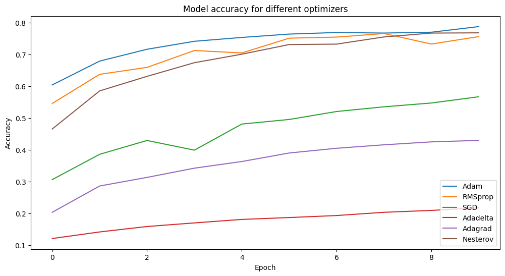
Visualization of the results 

Easily we can understand that Adam performs best, then Nesterov performs well, then RMSProp, then SGD, then Adagrad, Then Adadelta performs. You can experiment more with other optimization algorithms and can change hyperparameters(epochs, other) and visualize the results.

# Plot the comparison of results
import matplotlib.pyplot as plt
plt.figure(figsize=(12, 6))
for name, history in histories.items()
    plt.plot(history.history['val_accuracy'], label=name)
plt.title('Model accuracy for different optimizers')
plt.ylabel('Accuracy')
plt.xlabel('Epoch')
plt.legend()
plt.show()

Conclusion

Optimization algorithms play a crucial role in the field of deep learning to improve performance and model building. Today we gain knowledge of a lot of things about Optimization algorithms. We have known the concept of Optimization algorithms, the training process of optimization algorithms, The advantages and disadvantages of each optimization algorithm, the structure of each algorithm, and lastly a comparison in image classification problems. Hope the articles makes you a strong understanding of the core concept and necessary things about the Optimization Technique. For more knowledge, you need to update with the current developing optimization technique and their use cases of them. You may try to develop new optimization algorithms that may contain more features and advantages like faster convergence rate, more adaptability with hyperparameters, can use in many use cases, and so on. Thanks for reading the whole article. Hope this article may help in practicing Deep learning tasks.