- Introduction to Deep Learning
- Data Preprocessing for Deep Learning
- Convolutional Neural Networks
- Recurrent Neural Networks (RNNs)
- Long Short Term Memory (LSTM) Networks
- Transformers
- Generative Adversarial Networks
- Autoencoder
- Variational Autoencoders
- Diffusion Architecture
- Reinforcement Learning in Deep Learning
- Optimization Algorithms for Deep Learning
- Regularization Techniques
- Model Tracking and Accuracy Analysis
- Hyperparameter Tuning Techniques
- Transfer Learning
- Deployment of Deep Learning Models with REST API
- Deep Learning on Cloud Platforms
- Mathematical Foundations for Deep Learning
Hyperparameter Tuning Techniques | Deep Learning
A Hyperparameter is a type of parameter that is external to the model and controls the learning of the model. The value of the hyperparameter can’t be estimated from the data. They are often used in the process of setting up the learning algorithm. Setting perfect values for the hyperparameters is always tricky. It depends on the experiments, experience, and so on. Because of needed the tuning of the hyperparameters, we should achieve a lot of knowledge in this criteria. Today we will discuss the whole thing about Hyperparameter tuning Techniques step by step. Stay with us.
Before moving into the details of the article, let’s know the topics that we will learn today.
Introduction
Hyperparameters and their impacts
Manual Hyperparameter tuning
Grid Search
Random Search
Bayesian Optimization
Evolutionary Algorithms
Automated hyperparameter tuning libraries
Considerations and best practices
Conclusion
Let’s move to the specific topics and understand all the parts clearly.
Introduction
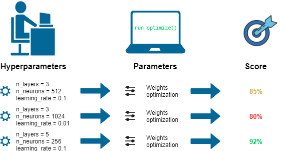
Hyperparameter is a variable that controls the behavior of the model. This variable is important to determine the structure of the model and the speed of learning. It should be set before starting the training process and remain constant throughout the training. The choice of hyperparameters can influence the model performance.
So it is very important to set the optimal values for the hyperparameter in the model. Like model parameters, hyperparameters can’t be learned from the training process, so we have to set it by ourselves. That’s why hyperparameter tuning comes in front of us.
The goal of hyperparameter tuning is to find the optimal values in the model. Finding the optimal values for the hyperparameter can be done in manual or systematic methods. Manual methods depend on experience, experiments, and so on. Systematic methods can be grid search, random search, bayesian optimization, and so on.
Let’s understand why the hyperparameter tuning methods are important in deep learning given below.
The goal of hyperparameter tuning is to improve the performance of the model. As an example, choosing the right learning rate in the optimization process can help to converge faster and avoid stacking in sub-optimal solutions. Choosing the right number of layers and a right number of neurons improve the model capacity and learn the complex patterns in the data.
By hyper-parameter tuning (dropout rate, regularization strength, model’s parameter), we can achieve a good balance between overfitting and underfitting.
Hyperparameters ( batch size and others) impact computational efficiency and memory efficiency. The batch size effect on the training speed and memory usage. So hyperparameter tuning is needed in this response.
The model complexity is often determined by its hyperparameter. A model with more layers and neurons is complex.
Hyperparameters such as learning rate, momentum, and optimizer choice can affect the learning dynamics of a model. They can affect faster learning and may perform sensitivity in noisy data and so on.
These are some examples of the importance of hyperparameter tuning in Deep Learning. Overall, hyperparameters determine the structure and learning process of the model, impact on model performance, computational efficiency, define model learning’s capability, and so on.
So, Finding the optimal set of hyperparameters is important for the overall success of the model. Experience and experiment with the hyperparameters are a key point for getting the optimal set of hyperparameters in Deep Learning.
Today, we will focus on the following process to find the optimal set of hyperparameters given below.
Manually hyperparameter tuning
Grid Search
Random Search
Bayesian Optimization
Evolutionary algorithms.
Let’s go forward to understand the whole concept of hyperparameter tuning.
Hyperparameters and their impacts
Hyperparameters are variables that control the structure, behavior of the model, and the way it learns from the data. They should set before starting the training process and not learn from the data during training. Now let’s learn about the role of hyperparameters in Deep Learning given below.
Some hyperparameters define the structure of the model such as the number of layers, the number of nodes in each layer, the type of layers(convolution, recurrent or other layers), activation functions, and so on.
Some hyperparameters control the learning process such as the learning rate determines how much the model’s weights will be updated, batch size determines the number of training examples used in one iteration to update the model weight, the number of epochs determines how many times the algorithm will work through the entire training dataset.
Some hyperparameters are used to control overfitting such as dropout rate, regularization methods, and so on.
Some hyperparameters can control the optimization process such as decay rate, momentum, and so on.
Overall, hyperparameters play a vast role in deep learning for various purposes. They impact model performance, robustness, and other utilities. So each of these hyperparameters must be tuned to find the best values for a specific problem. Let’s know some of the important hyperparameters that need to tune and apply to the model are given below.
The learning rate of an optimizer
Batch size
Number of layers and nodes in each layer
Activation functions
Weight initialization
Dropout rate
Momentum
Regularization parameters
Optimizer
Learning rate schedule/ decay
Early stopping
Gradient clipping
Number of filters, kernel size, pooling size
Loss function
Actually, the number of hyperparameters is huge. The important of them are listed above. Let’s understand how to tune the hyperparameters in various ways.
Manual Hyperparameter tuning
Tuning hyperparameters manually indicates adjusting hyperparameters by hand based on intuition, experience, and rules of thumb and observing how these adjustments affect model performance. Generally, it is the first approach to find the optimal set of hyperparameters.
Let’s understand how we can experiment with hyperparameter tuning manually given below.
Firstly understand what each hyperparameter does and how they impact model training and performance.
Start with default hyperparameter values that are provided by many machine learning libraries.
Once we have a baseline, then start adjusting hyperparameters one at a time.
Some hyperparameters have a large effect on model performance than others like learning rate. Tune these types of hyperparameters first.
Try to use a systematic approach to adjust the values manually.
Try to understand the relationship between hyperparameters and performance by monitoring the changes in model performance as well as hyperparameters.
After going through each hyperparameter, try to improve the model from the initial baseline.
The above Techniques can be taken to perform hyperparameter tuning manually. Manual tuning of each hyperparameter can be a good way to understand the effect of each hyperparameter on model performance. It has some advantages and disadvantages too. Let’s understand the pros and cons of tuning hyperparameters manually are given below.
Advantages/Pros of Manual Hyperparameter Tuning
It gives a better understanding of how different hyperparameters affect the performance of the model.
It does not require complex software or huge computational resources.
You can apply your insights and domain knowledge to complete the tuning process.
It gives full control over the tuning process and allows us to make informed decisions about trade-offs between model performance and complexity, training time, and so on.
Disadvantages/Cons of Manual Hyperparameter Tuning
This process can be slow. Especially when there are many hyperparameters to tune, then the process will be time-consuming.
Due to time constraints, you can explore a small subset of all possible hyperparameter combinations.
Manual tuning can occur fewer results compared to automatic tuning methods like grid search, random search, and so on.
The manual process may be influenced by bias.
At the time of tuning manually, it can be difficult to understand and manage these interactions manually.
Overall, Manual hyperparameter tuning may be a good way to start model building process but for optimal results, an automated tuning process can be good.
Grid Search
Grid Search is an automated method that is used for hyperparameter tuning in machine learning. The main idea of Grid Search is to set the possible values of each hyperparameter that you want to tune, then systematically try all combinations of these values to find the best ones.
Here the algorithm systematically trains a separate model for each combination of hyperparameters in the grid. Each model performance is evaluated on the validation dataset. The process is repeated for all combinations of hyperparameters. After completing the processes of all combinations, best-performing model is then selected for further work.
The process of searching hyperparameter combinations exhaustively in the grid search technique is given below.
Defining hyperparameters grid: first, it is needed to define the hyperparameters that will be tuned and the range of values for each of them. Suppose you want to tune the batch size and epochs hyperparameter of a deep learning model. Then the grid can be defined as {‘batch size’:[32,64,128], ‘epoch’:[30,50]}
Construct and evaluate a model for each combination: Now Grid Search constructs and evaluate a model for each combination of hyperparameters. The first combination will be batch size 32 and epoch 30, then the second combination will be batch size 32 and epoch 50, and the third will be batch size 64 and epoch 30 and continue. For each combination, it will run the model and evaluate performance on the validation dataset.
Selecting Best Hyperparameters: After completing the training of the model for all combinations, select the combination of hyperparameters that gives the best performance.
Re-Train the model: Now apply the best hyperparameters in the model to retrain with the entire dataset.
These are the overall process of Grid Seach methods. We can train and evaluate the model for each combination using the cross-validation technique to get a more robust model.
Evaluation of each combination of hyperparameters using cross-validation
Grid Search with cross-validation is an interesting approach to tuning hyperparameters in machine learning. For this approach, first, define a grid of hyperparameters to tune. Then for each combination of hyperparameters in the grid, you have to perform a cross-validation technique.
For cross-validation, split the entire data into a certain number of folds(5/10/others). For each combination, train the models for the number of fold times. For each time, one fold remains to evaluate and others for training the model and for different times, different fold will be used to evaluate the model. Then compute the average performance for all folds in each combination of hyperparameters. After completing the whole training, choose the best hyperparameter combinations for the model.
This is the process and it has some benefits such as it provides more robust estimates for the model’s performance. But this process is computationally more expensive than others. Now let’s learn about the advantages and disadvantages of Grid Search methods.
Pros of Grid Search
It tries all the possible combinations of the hyperparameters provided in the grid. So if the optimal set of hyperparameters is within the grid, grid search will find it.
The implementation of Grid Search is simple and straightforward.
It can be easily parallelized because each set of hyperparameters is independent to others.
It is easy to interpret and gives a clear understanding of the combinations of hyperparameters.
Cons of Grid Search
This method is computationally expensive and time-consuming.
Not all hyperparameters are equally important but grid search take all are the same.
As the number of hyperparameters increases, the number of combinations grows exponentially. This makes grid search inefficient for tuning a model.
Implementation of Grid Search
Tensorflow
You will get the code in Google Colab also.
import tensorflow as tf
from tensorflow.keras.wrappers.scikit_learn import KerasClassifier
from sklearn.model_selection import GridSearchCV
def create_model(optimizer='adam'):
    model = tf.keras.models.Sequential()
    model.add(tf.keras.layers.Dense(10, activation='relu', input_shape=(8,)))
    model.add(tf.keras.layers.Dense(1, activation='sigmoid'))
    model.compile(loss='binary_crossentropy', optimizer=optimizer, metrics=['accuracy'])

    return model
model = KerasClassifier(build_fn=create_model, verbose=0)
param_grid = {'batch_size': [10, 20, 50, 100],
              'epochs': [20, 50],
              'optimizer': ['adam', 'rmsprop']}
grid = GridSearchCV(estimator=model, param_grid=param_grid, n_jobs=-1)
grid_result = grid.fit(X, y)  # X and y are your data print("Best: %f using %s" % (grid_result.best_score_, grid_result.best_params_))
Pytorch
import torch
import torch.nn as nn
from sklearn.model_selection import GridSearchCV
from skorch import NeuralNetBinaryClassifier  # a sklearn-compatible neural network library that wraps PyTorch
class Net(nn.Module):
    def __init__(self):
        super(Net, self).__init__()
        self.fc1 = nn.Linear(8, 10)
        self.fc2 = nn.Linear(10, 1)
    def forward(self, x):
        x = torch.relu(self.fc1(x))
        x = torch.sigmoid(self.fc2(x))
        return x
net = NeuralNetBinaryClassifier(module=Net, max_epochs=10, lr=0.1, optimizer=torch.optim.SGD)
param_grid = {'max_epochs': [10, 20],
              'lr': [0.01, 0.1],
              'optimizer': [torch.optim.SGD, torch.optim.Adam]}
grid = GridSearchCV(estimator=net, param_grid=param_grid, cv=3, scoring='accuracy')
grid_result = grid.fit(X, y)  # X and y are your data
print("Best: %f using %s" % (grid_result.best_score_, grid_result.best_params_))
Random Search
Random Search is a hyperparameter tuning method that selects hyperparameter combinations randomly. The grid search method systematically explores all possible combinations of hyperparameters but the random search selects a combination of hyperparameters randomly and the model is trained on that combination and evaluated on a validation set and this is repeated until the maximum number of iterations is reached. Then select the best performer combination of hyperparameters. It is more computationally efficient than the Grid Search method.
Sampling hyperparameter combinations randomly
Now we are going to describe the whole process of the random search hyperparameter tuning method given below.
Firstly define which hyperparameters you want to tune and define the distribution or range for each hyperparameter and also have to define the number of iterations in the model that will be trained. Suppose the hyperparameter space can be {learning_rate:[0.1,0.01,0.001], epochs:[10,20,30]}
Now the algorithm randomly selects a value for each hyperparameter from its defined range or distribution and then forms a combination of hyperparameters. From the above hyperparameter space, it may be learning_rate: 0.01 and epochs: 30.
Then the model is trained on the chosen combination of hyperparameters and evaluated on a validation dataset.
The second and third steps will be repeated for the predefined number of iterations.
After completing the whole training process, choose the combination of hyperparameters that gives the best mode performance.
This is the overall process of the random search hyperparameter tuning method which samples hyperparameter combinations randomly.
Construct and evaluation of randomly selected combinations using cross-validation
This type of approach is discussed before in the grid search technique. Here the main difference is grid search select each combination sequentially and random search sampling each combination of hyperparameter randomly. After getting the combination of hyperparameters, performing cross-validation on that, and when the model reaches the maximum value of the number of iterations, you can choose the best-performing hyperparameter combination for the model.
Here just the method of choosing each combination of hyperparameters for training and evaluation is different and the other rest of the processes are the same.
Now let’s know about the advantages and disadvantages of random search hyperparameter tuning are given below.
Pros of random Search
Random search is more computationally efficient than Grid Search. We can find an optimal combination of hyperparameters in fewer iterations.
It is flexible to specify the hyperparameters as discrete or continuous.
Like Grid Search, this process is also parallelizable.
Cons of Random Search
No guarantee to find the optimal set of hyperparameters.
Like Grid Search, it can be computationally expensive and time-consuming.
Overall, It is more efficient than other hyperparameter optimization techniques. It can be a good starting point for hyperparameter optimization.
Implementation of Random Search
Tensorflow
import tensorflow as tf
from tensorflow.keras.wrappers.scikit_learn import KerasClassifier
from sklearn.model_selection import RandomizedSearchCV
from scipy.stats import uniform
def create_model(optimizer='adam'):
    model = tf.keras.models.Sequential()
    model.add(tf.keras.layers.Dense(10, activation='relu', input_shape=(8,)))
    model.add(tf.keras.layers.Dense(1, activation='sigmoid'))
    model.compile(loss='binary_crossentropy', optimizer=optimizer, metrics=['accuracy'])

    return model
model = KerasClassifier(build_fn=create_model, verbose=0)
param_dist = {'batch_size': [10, 20, 50, 100],
              'epochs': [20, 50],
              'optimizer': ['adam', 'rmsprop']}
random_search = RandomizedSearchCV(estimator=model, param_distributions=param_dist, n_iter=10, cv=3, random_state=42)
random_search_result = random_search.fit(X, y)  # X and y are your data print("Best: %f using %s" % (random_search_result.best_score_, random_search_result.best_params_))
Pytorch
import torch
import torch.nn as nn
from sklearn.model_selection import RandomizedSearchCV
from skorch import NeuralNetBinaryClassifier  # a sklearn-compatible neural network library that wraps PyTorch
from scipy.stats import uniform
class Net(nn.Module):
    def __init__(self):
        super(Net, self).__init__()
        self.fc1 = nn.Linear(8, 10)
        self.fc2 = nn.Linear(10, 1)
    def forward(self, x):
        x = torch.relu(self.fc1(x))
        x = torch.sigmoid(self.fc2(x))
        return x
net = NeuralNetBinaryClassifier(module=Net, max_epochs=10, lr=0.1, optimizer=torch.optim.SGD)
param_dist = {'max_epochs': [10, 20],
              'lr': uniform(loc=0, scale=0.1),
              'optimizer': [torch.optim.SGD, torch.optim.Adam]}
random_search = RandomizedSearchCV(estimator=net, param_distributions=param_dist, n_iter=10, cv=3, random_state=42)
random_search_result = random_search.fit(X, y)  # X and y are your data
print("Best: %f using %s" % (random_search_result.best_score_, random_search_result.best_params_))
Bayesian Optimization
It is a sequential model-based optimization that uses Bayesian methods to model the search space of optimization problems. It is used for the global optimization of black-box functions that do not require derivatives. It works by constructing a posterior distribution of functions(Gaussian process) that best describes the function that you want to optimize. As the number of observations increases, the posterior distribution improves, and the algorithm becomes more certain of which regions in parameter space are worth exploring and which are not.
The idea behind Bayesian Optimization is to treat the objective function as a random function and place a prior over it. The prior captures our beliefs about the properties of the function. After observing the function at a set of points, we update our prior into a posterior distribution. This posterior distribution over functions, combined with a utility function, then determines where to sample the function next.
Bayesian optimization has the ability to balance exploitation with exploration. Exploitation involves choosing points where the function value is high (according to the current model), while exploration involves choosing points where the uncertainty is high.
Mainly there are two components in Bayesian optimization that are given below.
A Surrogate model is used to approximate the unknown objective function. Gaussian Processes are usually used as surrogate models in Bayesian Optimization because they provide a measure of the uncertainty of predictions.
Acquisition Function that guides the selection of the next point to evaluate. It trades off between exploration and exploitation.
Balancing Exploration and Exploitation
Exploration involves searching the parts of the hyperparameter space that have not been sampled yet or where the model has high uncertainty. The aim of exploration is to gain more information about the objective function to potentially find better regions in the hyperparameter space. Exploitation involves sampling points in regions where the model predicts high performance, i.e., we believe the objective function value to be high. The aim of exploitation is to fine-tune the hyperparameters in the most promising regions of the hyperparameter space to achieve the best possible performance. When the acquisition function prioritizes points with high uncertainty, it encourages exploration and when the acquisition function prioritizes points with high expected performance, it encourages exploitation.
Different acquisition functions balance exploration and exploitation in different ways. Such as The Upper Confidence Bound (UCB) acquisition function includes an adjustable parameter that directly controls the balance between exploration and exploitation. The Expected Improvement (EI) acquisition function automatically balances exploration and exploitation based on the current state of the model and does not require an adjustable parameter. Striking a good balance between exploration and exploitation is crucial for the efficiency of Bayesian Optimization. Too much exploration can lead to wasting evaluations on poor hyperparameter configurations, while too much exploitation can lead to premature convergence to a local optimum.
Bayesian optimization has several advantages and disadvantages.
The advantages are given below-
It often finds better solutions with fewer function evaluations than grid search and random search.
It takes into account uncertainty in the model's predictions, which can lead to better exploration of the search space.
It has a good balance between exploration and exploitation.
It is designed for sequential decision-making, meaning it improves its understanding of the optimization problem with each new evaluation and no gradient is required.
The disadvantages are given below-
Bayesian optimization assumes that the objective function is smooth, which might not always be the case in practice.
it can still struggle with very high-dimensional spaces.
Bayesian inference can be quite computationally expensive.
The performance of Bayesian optimization can be sensitive to the choice of the prior and the kernel function used in the Gaussian process.
It can be affected by noisy evaluations of the objective function
Despite these limitations, Bayesian optimization is widely used for hyperparameter tuning in machine learning due to its efficiency and effectiveness.
Implementation of Bayesian Optimization
from hyperopt import hp, fmin, tpe, Trials, STATUS_OK
from sklearn import datasets
from sklearn.svm import SVC
from sklearn.ensemble import RandomForestClassifier
from sklearn.neighbors import KNeighborsClassifier
from sklearn.model_selection import cross_val_score
# Load the dataset
iris = datasets.load_iris()
X = iris.data
y = iris.target
# Define the search space
space = hp.choice('classifier_type', [
    {
        'type': 'naive_bayes',
    },
    {
        'type': 'svm',
        'C': hp.lognormal('svm_C', 0, 1.0),
        'kernel': hp.choice('svm_kernel', ['linear', 'rbf']),
    },
    {
        'type': 'random_forest',
        'max_depth': hp.choice('rf_max_depth', range(1,20)),
        'max_features': hp.choice('rf_max_features', range(1,5)),
        'n_estimators': hp.choice('rf_n_estimators', range(1,20)),
        'criterion': hp.choice('rf_criterion', ["gini", "entropy"]),
    },
    {
        'type': 'knn',
        'n_neighbors': hp.choice('knn_n_neighbors', range(1,50))
    }
]) # Define the objective function def objective(params):
    classifier_type = params['type']
    del params['type']
    if classifier_type == 'naive_bayes':
        clf = GaussianNB()
    elif classifier_type == 'svm':
        clf = SVC(**params)
    elif classifier_type == 'random_forest':
        clf = RandomForestClassifier(**params)
    elif classifier_type == 'knn':
        clf = KNeighborsClassifier(**params)
    else:
        return 0
    return -cross_val_score(clf, X, y, cv=5).mean() # Run the optimization trials = Trials()
best = fmin(objective, space, algo=tpe.suggest, max_evals=100, trials=trials)
print(best)
Evolutionary Algorithms
Evolutionary algorithms (EAs) are a type of optimization algorithm that is inspired by biological evolution. They use mechanisms of biological evolution such as selection, mutation, recombination (also known as crossover), and survival of the fittest to find optimal or near-optimal solutions to complex problems.
Let’s understand the working procedure of the evolutionary algorithms given below step by step.
Population Initialization: A set of potential solutions, referred to as individuals are randomly generated to form an initial population.
Fitness Evaluation: Each individual in the population is evaluated using a fitness function to determine how well it solves the problem at hand.
Selection: Individuals are selected, based on their fitness, to reproduce and generate offspring for the next generation. The better an individual's fitness, the higher their chance of being selected.
Crossover (Recombination): Selected individuals are paired up, and parts of their encoding are exchanged to produce offspring. This process allows the offspring to inherit traits from both parents.
Mutation: After crossover, the mutation is applied with a certain probability to introduce small changes. This helps maintain diversity within the population and prevents premature convergence to a suboptimal solution.
Survivor Selection: The offspring and the current population compete based on fitness, and only the fittest individuals survive to form the next generation.
Termination: This process is repeated until a satisfactory solution has been found or a preset condition is met, such as a maximum number of generations or a sufficient fitness level.
This is the overall process of evolutionary algorithms. Now let’s understand how to create a population of hyperparameter combinations.
Creating a population of hyperparameter combinations
It is a critical first step in hyperparameter tuning methods that use evolutionary algorithms or genetic algorithms. The purpose is to generate a diverse initial set of hyperparameters to explore different regions of the hyperparameter space.
The process of creating a population of hyperparameter combinations is given below.
The first step is to define the hyperparameters you want to tune and their possible values.
Once you have the hyperparameters and their ranges, you can generate random combinations of these values. Each combination represents a potential solution (an individual) in the population. The number of combinations you generate will be the size of your initial population.
Advantages and Disadvantages in Evolutionary Algorithms
Evolutionary algorithms (EAs) offer a unique and effective method for hyperparameter optimization in deep learning. The advantages of evolutionary algorithms are given below.
EAs are designed to find the global optimum in a search space and are less likely to get stuck in local minima compared to some other optimization methods.
EAs work well in complex, non-linear, and high-dimensional spaces.
Evaluations of different individuals are independent and can be parallelized across multiple CPUs or GPUs, which can significantly speed up the process.
EAs are generally robust to the choice of hyperparameters for the EA itself (like mutation rate and crossover rate).
EAs balance exploration (searching new areas) and exploitation (refining solutions in promising areas) effectively.
It has some limitations too. Some of them are given below.
It is Computationally Expensive.
It has no Guarantee of Optimal Solution.
Implementing EAs can be more complex than traditional methods like grid search or random search.
EAs usually require a large population of solutions, which might not be feasible for very large or complex models.
In summary, evolutionary algorithms offer a powerful method for hyperparameter optimization in deep learning, but they need to be used thoughtfully, considering the computational resources and time available.
Implement the Evolutionary Algorithms
!pip install deap
from deap import base, creator, tools, algorithms
import random
import numpy as np
from tensorflow.keras.models import Sequential
from tensorflow.keras.layers import Dense
from tensorflow.keras.optimizers import Adam
from sklearn.model_selection import train_test_split
from sklearn.metrics import mean_squared_error
# Assuming X and y are your data
X_train, X_test, y_train, y_test = train_test_split(X, y, test_size=0.2, random_state=42)
# Create the fitness and individual classes
creator.create("FitnessMin", base.Fitness, weights=(-1.0,))
creator.create("Individual", list, fitness=creator.FitnessMin)
# Define the individual and population classes
toolbox = base.Toolbox()
toolbox.register("attr_neurons", random.randint, 1, 100)
toolbox.register("attr_learning_rate", random.uniform, 0.001, 1)
toolbox.register("individual", tools.initCycle, creator.Individual,
                 (toolbox.attr_neurons, toolbox.attr_learning_rate), n=1)
toolbox.register("population", tools.initRepeat, list, toolbox.individual)
# Define the evaluation function
def evaluate(individual):
    model = Sequential()
    model.add(Dense(individual[0], input_dim=X_train.shape[1], activation='relu'))
    model.add(Dense(1, activation='linear'))
    model.compile(loss='mean_squared_error', optimizer=Adam(lr=individual[1]))
    model.fit(X_train, y_train, epochs=10, verbose=0)
    predictions = model.predict(X_test)
    return mean_squared_error(y_test, predictions),
toolbox.register("evaluate", evaluate)
toolbox.register("mate", tools.cxTwoPoint)
toolbox.register("mutate", tools.mutUniformInt, low=[1, 0.001], up=[100, 1], indpb=0.1)
toolbox.register("select", tools.selTournament, tournsize=3)
pop = toolbox.population(n=50)
hof = tools.HallOfFame(1)
stats = tools.Statistics(lambda ind: ind.fitness.values)
stats.register("avg", np.mean)
stats.register("min", np.min)
stats.register("max", np.max)
pop, logbook = algorithms.eaSimple(pop, toolbox, cxpb=0.5, mutpb=0.2, ngen=10, stats=stats, halloffame=hof, verbose=True)
Automated hyperparameter tuning libraries
There are several libraries that are used to perform automated hyperparameter tuning. These libraries provide a variety of tuning methods such as grid search, random search, bayesian optimization, and evaluation algorithms. Now we will discuss the features of each library, their advantages, and limitations of them.
Scikit-Learn: It is a popular Python library that provides GridSearchCV and RandomSearchCV functions with cross-validation for hyperparameter tuning. These functions are easy to use and integrate into sklearn pipelines. But Grid Search can be very computationally expensive for large hyperparameters. Random search can be computationally efficient but it may fail to get optimal hyperparameter values.
Keras Tuner: It is specially built for hyperparameter tuning for Keras models. It gives many hyperparameter techniques such as Random Search, Hyperband, and Bayesian Optimization. If you are using Keras Module, it can be a natural choice for hyperparameter tuning. Another option is, you can guild the hyperparameter tuning functions by the early stopping strategy. The main limitation is Keras tuner is only for Keras. If you are using another library, then you can’t use the Keras tuner.
HyperOpt: It provides two search algorithms(Tree of Parzen Estimators(TPE), and Random Search). It supports a variety of parameter expressions. It is designed for distributed, asynchronous optimization, so it can leverage parallel computing resources effectively. Hyperopt’s API can be complex and harder to learn than other libraries. This library doesn’t actively maintain. So, It can lead to issues with compatibility and bug fixes.
Optuna: It is a powerful library and can be used for hyperparameter tuning. It provides Tree-structured Parzen Estimator(TPE) and CMA_ES functions to optimize that support both numerical and categorical parameters. It provides a simple and user-friendly API and has visualization capabilities to make the optimization process interpretable and insightful. But it is more complex to use than basic tools like GridSearchCV and RandomSearchCV. It can be slow for large datasets but can be effective for finding optimal hyperparameters.
Ray Tune: It provides multiple tuning algorithms such as Grid Search, Random search, Bayesian Optimization, Hyperband, and Population Based Training(PBT). It can work well with many libraries like Pytorch, keras, tensorflow, sklearn, and many others. It can handle distributed computing. It can be integrated into many machine-learning libraries. It is a little complex in the setup and execution process.
There are many other libraries for automated hyperparameter tuning like TPOT, H2O’s autoML, Auto sklearn, and so on. These libraries provide automated hyperparameter tuning in the model to find the optimal set of hyperparameters. Automating hyperparameter tuning is a core concept in Deep learning. So, It is used in most of the fields of Deep Learning such as Computer Vision(Image classification, Image Segmentation, Object Detection, and so on), Natural Language Processing, Recommendation Systems, Fraud Detection, Autonomous vehicles, reinforcement learning, and so on.
Considerations and best practices
We have discussed a lot of things about hyperparameter tuning. But at the time of hyperparameter tuning, we should consider some items such as efficient resource utilization, handling large-scale and complex problems, setting the search space and hyperparameter distribution, and interactions between different hyperparameters and their effects of the performance and so on. Based on the consideration, we have to take the necessary steps to move forward.
Setting Search Space and hyperparameter distribution: The search space refers the possible values for each hyperparameter that the tuning process should consider. Suppose we want to tune the learning rate for the optimization process. So, for tuning I take 3 values (0.1,0.01,0.001). From the three values, we will find the optimal values for the learning rate. These three values are search space. When setting the search space, we should consider the trade-offs between wider search space and computational resources. A wider search space increases the chances of finding the optimal hyperparameters but takes more computational resources and time. A narrower search space may fail to find the optimal hyperparameters. So, it is needed to maintain the trade-offs.
For some hyperparameter tuning methods like Random Search, Bayesian Optimization, TPE, we have to define a distribution over the search space for each hyperparameter. Suppose for learning rate hyperparameter, you might define a log uniform distribution over the interval [0.0001,0.1] which means the lower learning rates are sampled more frequently than the higher ones. Another example is for the number of layers, you can use uniform distribution over the search space that indicates all number of layers are equally likely. Defining the hyperparameter distribution in the search space accurately can make the tuning process more efficient and can impact on the model performance also.
Efficient resource utilization during hyperparameter tuning: Hyperparameter tuning is a computationally expensive and time-consuming task. So some steps can be taken to efficiently utilize the resource during hyperparameter tuning. If you have multi-core machines or clusters of machines, you can run multiple hyperparameter configurations in parallel. We can use early-stopping strategies if the hyperparameter configurations can’t perform well. No need of using grid search for the first time, we can use random search, Bayesian Optimization, or gradient-based optimization which can provide good results in fewer trials. You can start with a large search space and progressively narrow down the search space based on the results of the initial stages. If you are tuning the hyperparameters for similar tasks/datasets, try to use the optimal hyperparameters which are getting from previous tasks. Prioritize important hyperparameters which have a big impact on the model performance. Before running extensive tuning on a large scale of data, a complex model, it can be beneficial to use a simple model on, a smaller dataset to quickly explore the hyperparameter space and identify promising regions.
Handling large-scale and complex problems: It is a complex task and challenging too. We can consider some strategies to solve the problem. First, we should consider distributed computing resources. To speed up the hyperparameter search process, we can run multiple trials in parallel. We can use efficient search algorithms such as Bayesian Optimization, TPE, Evaluation Algorithm and so on. In complex problems, it can be beneficial to use meta-learning or surrogate models.
You can also use early stopping methods to stop the training process.
Interactions between different hyperparameters and their effect on performance: Understanding the interactions between hyperparameters and their impact on performance are crucial for practitioners. It helps to guide the hyperparameter tuning process and improve model performance. Some hyperparameters impact more than others and sometimes two or more hyperparameters impact on We have considered those items and made an effective hyperparameter tuning process.
Conclusion
After a detailed discussion, we have reached the final topics of the tutorial. We have understood the concept of hyperparameter tuning Techniques, some tuning processes, and how to do tuning processes through various libraries, considerations, and best practices. Great we have covered all the parts based on Hyperparameter tuning. In the future, There are more processes have been developed. Be connect with them. Do experiment, experiment, and more experiments. Hope, you can understand the whole tutorial and enjoy the article. Thanks for reading the tutorial.