Mathematical Foundations for Deep Learning | Deep Learning

Learning Math is a requirement for mastering deep learning. This is due to the fact that deep learning relies heavily on mathematics at every stage, from selecting the right algorithm to altering the parameters. For this reason, a strong background in mathematics is essential to comprehending and using deep learning.

This article will discuss the mathematical concepts needed to study deep learning. Linear algebra, calculus, probability and statistics, and numeric computing are some of these areas. We will also talk about how mathematics is used in neural networks.

Linear Algebra for Deep Learning

Let’s talk about vectors, matrices, and tensors.

A vector has two properties, magnitude and direction. Using them, we can represent a single data point using a vector.

A vector can be described as an array of numbers with one dimension. It can be used to represent a set of features.

Vectors can be employed to symbolize:

• Data representations: Data are represented as vectors in various deep-learning applications. For instance, a vector of pixel values can be used to represent each image in image processing. This is what is known as feature representation.
• Neural Networks: Vectors may be used as the inputs and outputs of neural networks. For instance, a vector might be sent to the input layer. A vector of class probabilities could be produced by the output layer at the other end. Word embeddings can be represented as vectors in natural language processing.
• Weight Matrices: Weight matrices can be represented as vectors to represent the link between output and input properties in neural networks.
• Bias Terms: Along with input features, many deep learning models also include bias terms. They can be portrayed as vectors as well.

We import Numpy first. Numpy is utilized by the Python programming language. 

Additionally, they have a large library of complex mathematical operations to perform on these arrays. Large multi-dimensional arrays and matrices are supported by NumPy. You will get the code in Google Colab also.

#Import numerical python as numpy 

import numpy as np

Vector creation:

In this example, first, we declare a list, then we use the np.array method to convert the list to a vector

# Convert the Python list 'list_horizontal' into a NumPy array 'vector_horizontal' and print the array. 
list_horizontal = [4, 5, 6]
vector_horizontal = np.array(list_horizontal)
print(vector_horizontal)

The output gives a horizontal vector:

[4 5 6]

To create a vertical vector, we do the following:

# Convert the nested Python list 'list_vertical' into a NumPy array 'vector_vertical' and print the array. 
        [20],
        [30]]
vector_vertical = np.array(list_vertical)
print(vector_vertical)

list_vertical = [[10],

The output is:

[ [10]
  [20]
  [30] ]

Matrices

Matrices are a two-dimensional array of scalars. One dimension defines the rows, while the other defines the columns.

Matrices are fundamental tools used for deep learning purposes. 

Uses of a matrix in the Deep Learning domain:

• Convolutional Neural Networks: Matrices are used extensively in CNNs to represent filters as a matrix of weights.
• Optimization: In various optimization problems, it is used to represent the variables that are being optimized. 
• Weight matrices: In neural network training, weight matrices are learned to optimize the network's performance.
• Covariance matrices: In some applications, such as principal component analysis, covariance matrices are used to analyze the relationships between different variables in a dataset.

We can represent a matrix in numpy using a two-dimensional array.

# Create a 2x3 matrix using NumPy's 'array' function and print the matrix. 
Matrix = array( [ [ 1, 2, 3 ], [ 4, 5, 6 ] ] )
print(Matrix)

from numpy import array

Output:

[ [1 2 3]
  [4 5 6] ]

Tensors

They are one of the most essential data structures used in the Machine Learning domain. They can be considered containers or buckets for numerical data. Tensors have the following properties:

1. Rank- The rank of a tensor defines the number of axes of the tensor. The number of axes determines how many indices will be required to access a specific value in the multi-dimensional array.

Considering a matrix, the rank of a matrix will be two. Considering a vector, its rank will be one.

A scalar tensor will have a rank of zero.

2. Shape- The number of dimensions along each axes is determined by the shape. For example, the dimension of a square matrix may be (2,2).

3. Data Type- Data types supported by tensors include:

• float32

• float64

• int32

• Int64

• uint8

Example of a tensor:

# Create a 3-dimensional NumPy array (tensor) and initialize it with the specified values. 
   [ [ 1,2, 3 ],    [ 4,5,6 ],    [ 7,8,9 ] ],
  [ [ 11,12,13 ], [ 14,15,16 ], [ 17,18,19 ] ],
  ] )

Tensor = array( [

Here we have declared a tensor of Shape (2,3,3)

Matrix Multiplication

Matrix multiplication is an important operation in deep learning.

The rules are as follows for multiplying two matrices, A and B.

• The column size of matrix A must equal the row size of matrix B to make the column sizes compatible.

• The multiplication of AB is not equal to that of BA. Hence it is not a commutative operation.

Example of Matrix Multiplication

# Define two 2-dimensional NumPy arrays 'A' and 'B' with the specified values. 
B=np.array([[90,80,70],[60,50,40]],ndmin=2) 

A=np.array([[10,20,30],[40,50,60]],ndmin=2)  

The administrator determines the minimum number of dimensions the array should have. One will be appended to the statement if needed to meet the requirement.

Next, we use the matmul functionality of numpy

# Multiply the NumPy arrays 'A' and 'B' element-wise and store the result in 'result'. 
result  

result = np.multiply(A,B)  

Output:

array( [ [ 900, 1600 , 2100]
            [2400, 2500, 2400] ] )

Dot product

To put it simply, the dot product between two vectors is the sum of the products of their corresponding elements.

The dot function of numpy is responsible for the dot product operation:

# Import the 'numpy.matlib' module to create matrices.
import numpy as np
# Define two 2x2 matrices 'A' and 'B' using NumPy arrays.
A = np.array([[1, 2],
              [3, 4]])
B = np.array([[5, 6],
              [7, 8]])
# Perform matrix multiplication between matrices 'A' and 'B' using 'np.dot()'.
result = np.dot(A, B)
# Print the result of matrix multiplication.

The output:

[ [ 19 22 ]
  [ 43  50] ] 

The primary difference is that, while matrix multiplication produces a new matrix whose size depends on the dimensions of the input matrices, dot product produces a scalar value. In linear algebra, these operations have distinct functions and are not equivalent.

Vector Norms

To put it simply, the length or magnitude of a vector is defined by vector norms. This norm is usually used to evaluate errors in deep learning models. Its functionality includes mapping a vector to a positive value. 

Some useful vector norms are:

L1 Norm aka the Manhatten Norm- L1 Norm measures the absolute value of each component of the vector. After that, those values are summed up to get the final value.

Example:

# Calculate the L1 (Manhattan) norm of the NumPy array 'A' and print the result. 

A = np.array([-1, 2, 3, 4, -5])
l1_norm_calculation = np.linalg.norm(A, ord=1)
print(l1_norm_calculation)

The output : 

15.0 

Here the output is the sum of the absolute value of each element 1+2+3+4+5=15

L2 norm or the Euclidean norm- measures the square root of the sum of the squares of the components of the vector.

# Calculate the L2 (Euclidean) norm of the NumPy array 'A' and print the result. 
l2_norm_calculation = np.linalg.norm(A,  ord=2)
print(l2_norm_calculation)

A = np.array( [-1, 2, 3, 4, -5] )

The output: 

7.416198487095663

Here the output is calculated as sqrt((-1)  2 + (2)2 + (3)2 + (4)2 + (-5)2) = 7.4162

Matrix Norms

Matrix norms can be considered functions that map a matrix to a non-negative scalar value. The most commonly used matrix norm in deep learning is the Forbenius norm. It measures the square root of the sum of the squares of all the elements in the matrix.

Example:

# Calculate the Frobenius norm of the NumPy matrix 'A' and print the result. 
forbenius_norm = np.linalg.norm(A, ord='fro')
print(forbenius_norm)

A = np.array( [ [1, 2, 3], [-1, -2, -3 ] ] )

The output:

5.291502622129181

Here the output was calculated as sqrt(12 + 22 + 32 + (-1)2 + (-2)2 + (-3)2) = 5.2915

Matrix Inversion

In this operation, we find the inverse of a matrix. This matrix, multiplied by the original matrix, will produce the identity matrix.

We use the linalg.inv function to achieve this in numpy:

# Compute the inverse of the 2x2 NumPy matrix 'A' and print the result. 
A_inverse = np.linalg.inv(A)
print(A_inverse)

A = np.array( [ [ -1, 2], [-3, 4 ] ] )

The output: 

   [[ 2.      -1. ]    
   [ 1.5    -0.5 ]]

Keep in mind a matrix is invertible if it’s determinant is non-zero

Matrix Determinant

Simply put, for a matrix like-

a b
c d

Determinant is calculated as determinant = ad-bc

This property of matrices is useful for various applications of linear algebra, such as 

Solving linear system equations or calculation of eigenvalues and eigenvectors

We can find the determinant using numpy using np.linalg.det:

# Compute the determinant of the 2x2 NumPy matrix 'A' and print the result. 
determinant_A = np.linalg.det(A)
print(determinant_A)

A = np.array( [ [ -1, 2 ],  [ 3, -4 ] ] )

Output:

-2.0000000000000004

EigenValue and EigenVector

EigenValue and EigenVectors are used to study the properties of a square matrix in linear algebra.

To simplify:

For the same matrix A

a b
c d

If we consider v to be an eigenvector of A, then

Av = λv

If we expand the equation, we get-

a*v[0] + b*v[1] = λ*v[0]
c*v[0] + d*v[1] = λ*v[1]

EigenValues and EigenVectors have several important properties:

• The sum of eigenvalues of a matrix is equal to the sum of diagonals of the matrix

• The product of eigenvalues equals its determinant

Eigenvalues and eigenvectors in numpy

# Calculate the eigenvalues and eigenvectors of the 2x2 NumPy matrix 'A' and print the results. 
eigenvalues, eigenvectors = np.linalg.eig(A)
print("Eigenvalues: ", eigenvalues)
print("Eigenvectors: \n", eigenvectors)

A = np.array( [ [ -1, 2 ],  [ 2, -1 ] ] )

Output: 

Eigenvalues:  [ 1   -3 ]
Eigenvectors:
  [ [  0.70710678   -0.70710678 ]
    [  0.70710678    0.70710678 ]]

Calculus for Deep Learning

Limits and Derivatives

Limits describe how a function behaves, as the input approaches a value. 

It can be used in Neural Networks to analyze its input behavior with changes in input

Limit in numpy:

# Define the function 'f(input)' and calculate the limit as the input approaches zero.
import numpy as np
def f(input):
    return np.sin(input) / input
# Create an array 'input' with 1000 equally spaced points from 0.001 to 1.
input = np.linspace(0.001, 1, 1000)
# Calculate the output of the function 'f' for each point in 'input'.
output = f(input)
# Find the maximum absolute value in the 'output' array and round it to 5 decimal places.
limit = np.around(np.max(np.abs(output)), decimals=5)
# Print the calculated limit.
print("The limit is:", limit)

Output: 

The limit is: 1.0

Here, we define a function f(input) that we want to find the limit of as input approaches 0. An array input is then created that contains 1000 evenly spaced values between 0.001 and 1. We use this array to evaluate f(input); the result is stored in output. Finally, the maximum absolute output value is rounded to 5 decimal places to approximate the limit.

Derivatives play an important role in optimizing weights and biases during the training of neural networks.

In calculus, we can define derivative as the rate of change of a function output in response to the input.

Numpy derivative function:

# Compute the numerical gradient of the data points represented by arrays 'x' and 'y' and print the result.
import numpy as np
# Define the array 'x' with the input data points.
x = np.array([0, 1, 2, 3, 4])
# Define the array 'y' with the corresponding output data points.
y = np.array([0, 10, 40, 90, 160])
# Compute the numerical gradient using 'np.gradient()' with respect to 'x'.
result = np.gradient(y, x)
# Print the resulting gradient values.
print(result)

We use the gradient function to achieve the result. Here the result is the derivative of y with respect to x.

Output: 

[ 3   432    27  48    675 ]

Product Rule

According to the product rule, if f(x) = g(x)h(x), 

                                                then f'(x) = g'(x)h(x) + g(x)h'(x)

In NumPy, we use numpy.multiply to achieve this

# Calculate the gradient of the function 'f(x)' and print the result.
import numpy as np
# Define the array 'x' with input data points.
x = np.array([2, 3, 1])
# Define the function 'u(x)' as 'x' squared.
u = np.power(x, 2)
# Define the function 'v(x)' as the sine of 'x'.
v = np.sin(x)
# Calculate the gradient of 'u(x)' with respect to 'x'.
u_grad = np.gradient(u)
# Calculate the gradient of 'v(x)' with respect to 'x'.
v_grad = np.gradient(v)
# Calculate the gradient of the function 'f(x) = u(x) * v(x)' using the product rule of derivatives.
f_grad = np.add(np.multiply(u_grad, v), np.multiply(u, v_grad))
# Print the resulting gradient values.
print(f_grad)

Output:

[  1.473777746    -0.516899    -6.0314169 ]

Chain Rule

In NumPy, we use the gradient function. This function applies the chain rule, resulting in the calculation of a composite function.

Example:

# Define three functions 'f(x)', 'g(x)', and 'h(x)', calculate their gradients, and print the result.
import numpy as np
# Define the function 'f(x)' as the sine of 'x' squared.
def f(x):
    return np.sin(np.power(x, 2))
# Define the function 'g(x)' as 'x' cubed.
def g(x):
    return np.power(x, 3)
# Define the function 'h(x)' as the composition of 'f(g(x))'.
def h(x):
    return f(g(x))
# Define the input data points 'x'.
x = np.array([1, 2, 3])
# Calculate the gradient of 'g(x)' with respect to 'x'.
g_grad = np.gradient(g(x))
# Calculate the gradient of 'f(g(x))' with respect to 'x' using the chain rule of derivatives.
f_grad = np.gradient(f(g(x)))
# Calculate the gradient of the composite function 'h(x) = f(g(x))' by multiplying the gradients of 'f' and 'g'.
h_grad = np.multiply(g_grad, f_grad)
# Print the resulting gradient values.
print(h_grad)

Output:

[  0.54988537   -4.49497209    -14.6316952 ]

Neural Network Optimization

We find a function's maximum and minimum values using the optimization technique. The gradient descent algorithm utilizes derivatives to find these minimum and maximum values.

Gradient descent starts with the initial value of a function. It then updates the value by taking the direction of the negative gradient of the function. Gradient Descent is used for updating the weights of neurons in neural network

# Perform gradient descent optimization to find the minimum of the function 'f(x) = x^2 - 2*x + 1'.
import numpy as np
# Define the function 'f(x) = x^2 - 2*x + 1'.
def f(x):
    return np.power(x, 2) - 2*x + 1
# Define the derivative of 'f(x)' as 'f_grad(x) = 2*x - 2'.
def f_grad(x):
    return 2*x - 2
# Set the learning rate for gradient descent.
learning_rate = 0.1
# Define the number of iterations for gradient descent.
iterations = 100
# Set the initial value for 'x_value'.
x_value = 5
# Perform gradient descent for the specified number of iterations.
for i in range(iterations):
    # Calculate the gradient of 'f(x)' at the current 'x_value'.
    df_dx = f_grad(x_value)
    # Update 'x_value' using gradient descent.
    x_value = x_value - learning_rate * df_dx
# Print the final value of 'x_value' after gradient descent.
print(x_value)

Here we define f(x) and the f_grad function, declare the learning rate and the number of iterations, and then update the value x_value using gradient descent for the specified number of iterations.

Integrals

Integrals are essential in deep learning for various applications, like Bayesian modeling. For example, integrals are required for calculating the posterior probabilities over the parameters of the model.

Example of integrals in NumPy

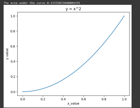
# Define the function 'f(x) = x^2' and calculate the area under the curve.
import numpy as np
import matplotlib.pyplot as plt
# Define the function 'f(x) = x^2'.
def f(x):
    return np.power(x, 2)
# Generate an array 'x' with 100 equally spaced points from 0 to 1.
x = np.linspace(0, 1, 100)
# Calculate the corresponding 'y' values using the function 'f(x)'.
y = f(x)
# Plot the curve of the function 'f(x)'.
plt.plot(x, y)
# Add labels and a title to the plot.
plt.xlabel('x_value')
plt.ylabel('y value')
plt.title('y = x^2')
# Calculate the area under the curve using the trapezoidal rule.
area = np.trapz(y, x)
# Print the calculated area.
print(f"The area under the curve is {area}")
# Show the plot.
plt.show()

Here we are trying to find the integral over x2

Output:

The area under the curve 0.33335033840084355

Probability and Statistics for Deep Learning

Some basic concepts

Random Variables: The possible values of a random variable are determined by a random event’s outcome. There are two types: Discrete random variables can take countably infinite or finite sets of values. For example, if we roll a die, the outcome is a discrete random variable. Another type is a continuous variable. It can take any variable within a given interval, like a person's height.

x = np.random.rand()
print(x)

It provides a random number between 0 and 1

Output:

0.7298877490762676

Distributions: Distribution describes how a random variable’s possible outcomes are distributed. Distributions are also of two forms: discrete and continuous. There are several types of distributions, such as Normal Distribution, Poisson Distribution, etc. Distributions are used in ML and DL for modeling uncertainty and variability in data. The distributions mentioned above are used to model the probability distributions of various random variables, such as inputs, outputs, weights, and biases, in the field of deep learning.

For example, a normal distribution is a bell-shaped curve. This curve is used to model the distribution of errors and noise in data. Another distribution is the gamma distribution.

Gamma Distribution: Positive real numbers (such as durations or counts) are frequently modeled using the gamma distribution, a continuous distribution. In Bayesian deep learning, it is frequently utilized as a prior distribution.

x = np.random.normal ( 0, 1, size=10 )
Print( x )

In this example a random sample from a normal distribution with a standard deviation of 1 and a mean of 0.

Output:

[ 067364062   -0.55241697   -0.89406081   0.87619116   0.45941227   2.67978362
1.4705075    -0.19844185     0.41875279      1.36734152  ]

Bayes’s Theorem

It is a famous theorem that represents the relationship between conditional probabilities. The theorem states that the probability of a hypothesis H given some observed evidence E is proportional to the probability of the evidence given the hypothesis, multiplied by the prior probability of the hypothesis. Symbolically, it can be written as-

where P(H | E) = posterior probability of the hypothesis given the evidence. P(E | H) = likelihood of the evidence given the hypothesis; P(H) = is the prior probability of the hypothesis, and P(E) is the marginal likelihood of the evidence.

Statistical concepts

Mean- To put it simply, the mean is the acreage value amongst a set of values.

# Calculate the mean (average) of the values in the NumPy array 'values' and print the result.
import numpy as np
# Define the NumPy array 'values' containing the data.
values = np.array([1, 2, 3, 4, 5])
# Calculate the mean of the values in the array using 'np.mean()'.
mean = np.mean(values)
# Print the calculated mean.
print("Mean:", mean)

Output: 

Mean: 3.0 

Variance: it is a measurement of how much deviation the data have from the mean

# Calculate the variance of the values in the NumPy array 'values' and print the result.
import numpy as np
# Define the NumPy array 'values' containing the data.
values = np.array([1, 2, 3, 4, 5])
# Calculate the variance of the values in the array using 'np.var()'.
variance = np.var(values)
# Print the calculated variance.
print("Variance:", variance)

Output:

Variance:  2.0 

Covariance: a measure of how two values vary or differ together.

# Calculate the covariance between 'x_value' and 'y_value' and print the result.
import numpy as np
# Define the arrays 'x_value' and 'y_value' containing the data points.
x_value = np.array([1, 2, 30, 4, 5])
y_value = np.array([2, 4, 60, 18, 10])
# Calculate the covariance matrix using 'np.cov()'.
covariance = np.cov(x_value, y_value)
# Print the covariance matrix.
print("Covariance:")
print(covariance)

Output:

Covariance:
[ [ 145.3   285.6 ]
  [ 285.6   569.2 ] ] 

Correlation: It is a measurement of the linear relationship between two variables in terms of strength and direction. 

Here, the covariance between x and y is divided by the product of their standard deviations.

# Calculate the correlation coefficient between 'x_value' and 'y_value' and print the result.
import numpy as np
# Define the arrays 'x_value' and 'y_value' containing the data points.
x_value = np.array([1, 2, 3, 4, 5])
y_value = np.array([2, 4, 6, 8, 10])
# Calculate the correlation matrix using 'np.corrcoef()'.
correlation = np.corrcoef(x_value, y_value)
# Print the correlation matrix.
print("Correlation:")
print(correlation)

Output: 

Correlation:
  [  [ 1. 1. ]
     [ 1.1.  ]  ]

Probability Distributions Used in Deep Learning

Gaussian Distribution: It is one of the most commonly used distributions in deep learning. It uses the mean and standard deviation to form the distribution. Its main use case is in modeling real-valued data.

Where 

=Standard Deviation

=mean

The code for Gaussian distribution has been given in the distribution section.

Bernoulli Distribution

It is a discrete probability distribution. Bernoulli Distribution models the probability of a binary outcome (0 or 1) in a single trial. It is used to model binary classification problem

# Generate 1000 random samples from a Bernoulli distribution with p=0.7
samples = np.random.binomial(1, 0.7, 10)
print(samples)

Output: 

[ 1 1 1 1 0 0 1 0 0 1 ]

We can use the binomial function of numpy with a number of trials set to 1

Poisson Distribution

It is a discrete probability distribution that models the probability of an event occurring among k possible outcomes.

In Numpy we can achieve this using:

samples = np.random.poisson(5, 10)
print(samples)

Output:

[ 6 5 3 7 2 2 9 4 3 5 ]

Hypothesis Testing

It is a statistical technique used to draw conclusions about a population parameter based on sample data. In this kind of testing, the null and alternative hypotheses are presented at the outset.

The null hypothesis implies there is no relationship between a sample statistic and a population parameter. 

The alternative hypothesis is the opposite of that. We use sample data to determine whether to reject the null hypothesis or not.

Statistical significance is a way to determine whether or not the results achieved from a machine learning model are meaningful. Statistical significance is assessed by hypothesis testing.

The process involves

• Selecting a test statistic

• setting a significance level 

• calculating a p-value

• comparing the p-value to the significance level to make a decision

Here p-value= = The probability of observing a test statistic as extreme as, or more extreme than, the one calculated from the sample data, assuming the null hypothesis is true.

We can do hypothesis testing using the t-test which is used to determine if two groups of data are significantly different from each other or not.

Here we use the scipy library to import stats library

# Perform an independent two-sample t-test to compare the means of 'sample1' and 'sample2'.
from scipy import stats
import numpy as np
# Generate two sets of sample data using random normal distribution.
sample1 = np.random.normal(0, 1, 10)
sample2 = np.random.normal(1, 1, 10)
# Calculate the test statistic (t-value) and p-value using the t-test.
t_value, p_value = stats.ttest_ind(sample1, sample2)
# Set the significance level (alpha).
alpha = 0.05
# Compare the p-value to the significance level to make a decision.
if p_value < alpha:
    print("Reject the null hypothesis")
else:
    print("Cannot reject the null hypothesis")

Output:

Cannot reject the null hypothesis

Numerical Computing for Deep Learning

Floating Point representation represents a real number in a binary format. In this format, the real number can now be stored and manipulated by a computer.

There are three parts to this format:

• A sign bit

• An exponent

• A mantissa (fraction)

Due to the finite number of bits allocated to mantissa and exponent, it can introduce to round-off errors.

For example, consider the decimal number 0.1. In binary representation, this number is expressed as a repeating sequence of bits (0.00011001100110011001100110011...). Since the number of bits in the mantissa is finite, we must eventually round off this sequence. However, this can introduce round-off errors, which can accumulate over multiple operations.

To mitigate the errors techniques can be performed like Numeric Normalization, Stabilization, etc.

For a 64-bit floating point representation we can write the following 

arr_float64 = np.array([[1.0, 2.0], [3.0, 4.0]], dtype=np.float64)
print(arr_float64)

Output:

[ [ 1.  2. ]
  [3.   4. ]]

Numeric Stability

Numerical stability refers to the ability of an algorithm or computation to produce accurate results in the presence of round-off errors and other numerical inaccuracies. A numerically unstable algorithm or computation can amplify these errors, leading to incorrect or nonsensical results. 

Numerical conditioning, on the other hand, refers to the sensitivity of an algorithm or computation to small changes in the input or parameters. A well-conditioned algorithm or computation is able to produce accurate results even when small changes are made to the input or parameters. A poorly conditioned algorithm or computation, on the other hand, can produce large errors or inaccuracies even with small changes to the input or parameters.

To improve numeric stability and conditioning, techniques used involve-

1. Numerical precision: Increasing precision can help reduce round-off errors

We can increase precision using Numpy:

# Create an array of 32-bit floats
arr_float32 = np.array([1.0, 2.0, 3.0], dtype=np.float32)
print(arr_float32)
# Create an array of 64-bit floats
arr_float64 = np.array([1.0, 2.0, 3.0], dtype=np.float64)
print(arr_float64)

Output:

 [  [ 1. 2. 3. ]
    [ 1. 2. 3. ]]

2. Numerical normalization: Normalizing input data can also increase numeric stability and conditioning.

# Create a 2D array
arr = np.array([[1, 2], [3, 4]])

# Calculate the L2 norm of the array
norm = np.linalg.norm(arr)
print(norm)

# Normalize the array by dividing each element by the norm
arr_normalized = arr / norm
print(arr_normalized)

Output:

5.477225575051661
[ [ 0.18257419        0.36514837 ]
   [0.54772256        0.73029674  ] ]

Numerical Integration

Numerical integration involves approximating the definite integral of a function over a given interval. 

def f(x):
    return np.exp(-x**2)
# Define the interval over which to integrate the function
x = np.linspace(-10, 10, 100)
# Use the trapezoidal rule to approximate the definite integral
integral_trapz = np.trapz(f(x), x)
print(integral_trapz)

Output: 

1.772453850955159

Here we used the trapezoidal rule for approximating the definite integral

Numerical Optimization

Numerical optimization involves finding the maximum or minimum of a function.

# Use the `minimize()` function to find the minimum of the function.
from scipy.optimize import minimize
import numpy as np
# Define the function to be minimized.
def f(x):
    return x[0]**2 + x[1]**2 + x[2]**2
# Define the initial guess for the optimal parameters.
x0 = np.array([1, 22, 30])
# Use the `minimize()` function to find the optimal parameters.
res = minimize(f, x0)
# Print the optimal values of the variables and the minimum value of the function.
print("Optimal Parameters:", res.x)
print("Minimum Value of the Function:", res.fun)

Application of Mathematics in Neural Networks

Basic structure of Neural Networks

A neural network is a machine-learning model that mimics the functionality of the human brain.

It consists of three components:

• Input layer: Responsible for receiving input data

• Hidden layer(s): Takes input from the input layer, transforms data, passes data to output layer

• Output layer: Produces output predictions

Activation Functions

They introduce non-linearity to neural networks, allowing neural networks to learn complex relationships between input and output.

Different types of activation functions include

Sigmoid function

Maps values between 0 and 1

def f(x):
  return 1 / (1 + np.exp( -x ) )

Rectified Linear Unit (ReLU)

Leaves positive values unchanged, and changes negative values to 0.

def relu(x):
  return max( 0, x)

Softmax 

Maps output values between 0 and 1. The sum of all values is 1. Used for multi-class classification.

def softmax(x):
    exp_x = np.exp(x)
    return exp_x / np.sum(exp_x)

It calculates the exponent of each component and then divides the exponent by the sum of the exponents of the components.

Backpropagation

It is popular for training deep neural networks. Simply put, it is used to calculate the gradients of the loss function with respect to the weights present in the neural network using gradient descent.

It has two phases:

Forward Propagation

• Input is provided to the neural network, and the output is computed

• Loss is calculated after comparison with target output

Backward Propagation

Using the chain rule of calculus. the gradient of the loss function with respect to the weights of the neural network is computed.

Gradient with respect to the loss of function.

dL/dw = (dL/dy) * (dy/dw) 

The gradients of the composite functions are calculated by multiplying the gradients of their individual components.

Applications of Linear Algebra and Calculus in Neural Networks

Backpropagation: Linear algebra is used to compute gradients and loss functions in backpropagation. The process of backpropagation involves gradient descent, which is a 

technique that can be used to update the weights and biases during learning. The gradient of the loss function can be determined using the chain rule of calculus. Matrix operations can be used to execute this computation, enabling parallel processing and quick memory access.

Convolutional neural networks: CNNs are deep learning neural networks that use convolutional layers to compute convolutional operations between input and learnable filters.

Essentially, CNN depends on convolution, which involves filtering the input image. It also performs the dot product operation between filter weights and corresponding pixel values in each spot.

Recurrent neural networks: RNNs work with sequential data that involves complex matrix multiplication. The main purpose of RNNs is to pass information from one sequence to the next using hidden states. These hidden states can be represented as vectors.  RNN also goes through the process of backpropagation, which uses matrix operations, as mentioned above.

Applications of Numeric Computing in Deep Learning

Matrix operations: Neural networks require lots of matrix operations like matrix multiplication, vector addition, etc. which libraries like NumPy provide. Here Numeric Computing has a deep impact on these deep learning applications. As discussed before, neural networks require procedures like gradient optimization, forward propagation, and backward propagation, matrix operations are vital for these purposes

Data preprocessing: Numeric computing plays a crucial role in data preprocessing tasks like data cleaning, normalization, and transformation.  These libraries allow efficient manipulation of large datasets. Along with this it also allows the conversion of data into a suitable format for neural network training.

Conclusion

This tutorial covered various mathematical concepts used in machine learning and deep learning domains. We covered topics ranging from linear algebra to numeric computing. We understood the concepts and also implemented them using Numpy. We also discussed the role of linear algebra and numerical computing for deep learning.

It is essential to have a good grasp of these mathematical concepts and practice them to prepare yourself for tackling deep learning and machine learning problems.