Transfer Learning | Deep Learning

Put simply, transfer learning is the process where a model developed for a specific purpose is reused as the starting point for another problem related to the first problem. In other words, it uses a pre-trained model to solve a new task. This allows deep neural networks to be trained with less data.

In this tutorial, we will cover the fundamentals of transfer learning. Next, we will look at how to prepare data for transfer learning and how to build a base model and fine-tune a pre-trained model. After that, we will apply transfer learning to the CIFAR-10 dataset. We will then discuss evaluation and testing methods for transfer learning, case studies and examples, and tips and best practices.

Fundamentals of Transfer Learning

In this process:

• A base dataset is used to train the base network

• The learned features from the base network are then transferred to a second target network

• The target, related, or unrelated dataset is then used to train the second network.

This system works if the learned features from the base network are generalized features. This means features learned will also benefit the target network, rather than only benefiting the base network. In this way transfer learning allows knowledge learned from the base network to generalize the target network. You can learn more here.

Different types of transfer learning

Develop Model approach

• In this approach, we first select a related problem. The related problem should have an abundance of data. Also, there should be some relationship between the input data while mapping input data to output data during learning.

• Next for the first problem, we develop a model which should perform better than a naive model. This will confirm that some feature learning has taken place.

• The source model now can be used for the second problem as the starting point. Depending on the use case the whole model can be used or only parts of the model can be used.

• If required, the model may need to be refined.

Pre-trained model approach

• Many research institutions release models trained on large datasets. We choose a pre-trained model from available models as the source model.

• As before it can then be used as the starting point of the second problem. Either full or partial parts of the model are used as required.

• Optionally the model may need to be refined when required on the input-output pair data.

Benefits of transfer learning include:

• We don’t require large amounts of labeled data to train our new model every time. Less labeled data is now required to get the same model performance saving time and resources.

• Efficiency for developing and deploying multiple models increases.

• Models can now be developed in an iterative fashion as knowledge can be shared between models.

• It solves the overfitting problem as now models can be trained on small datasets, using these pre-trained models, without overfitting.

Preparing data for transfer learning

Data preparation is crucial for the transfer learning process. The quality of data has a significant effect on the performance of a model. By ensuring the source model is trained on high-quality data, we can improve the performance of the target model subsequently.

What type of data is chosen for the source model also matters in the case of transfer learning. The dataset the source model learns on is relevant to the target network. It is better if the source network dataset is a generalized dataset, as it would help the model learn generalized features, which in turn will benefit the target network. 

Preprocessing data for transfer learning

To increase efficiency, we can take the following steps:

• Remove irrelevant and duplicate data- removing data not required for learning is essential for smooth and faster learning. It ensures features learned are relevant.

• Data Augmentation- This is where new data is created from the transformation of original data. In terms of images this can involve flipping, rotating, zooming, or cropping them. This increases the diversity of the training set, which can lead to a more robust model

• Data Normalization- Data normalization involves scaling data so that input features have the same scales and the model can be trained efficiently.

• Encoding categorical values- If categorical variables is required, one hot encoding or label encoding can be carried out to encode the variables in a way the transfer learning model can process.

• Removing outliers- removing outliers can help the source model train on representative data.

Example of data preprocessing

If we consider preprocessing an image for training we can do the following:

Resize the image: If we are looking to use a pre-trained model VGG16 on a new dataset, it expects the images to be of size 224x224 pixels, hence the images can be resized to train the model.

Data Augmentation: Augmentation techniques like rotation, translation, and horizontal flip can be applied to the images, which in turn increases the diversity of the training dataset.

Normalization: All the pixel values of the images can be normalized by dividing their value by 255 so that all the pixel values are between 0 and 1.

Removing outliers: If any images are corrupted or represent irrelevant classes, they can be removed.

Building a base model

This requires the following steps:

• Choosing a pre-trained model: The first step is to choose a pre-trained model that is trained on a large dataset. There are several popular models to choose from, such as CNN models like VGG16, Resnet, or Inception. The choice depends on the size of the dataset and the nature of the task.

• Remove the top layers: There are several layers present on the pre-trained model which were specific to the original task when the model was trained. We need to remove these top layers. They usually include final output layers and fully connected layers that follow them. 

• Freeze the pre-trained layer: The pre-trained layers should not be updated during the training process. The model should only learn from the layers which are added on top of the pre-trained layers. Hence, these layers must be frozen before training.

• Add new layers: New layers suitable for the specific target task should be added on top of the pre-trained layers. For example, for image classification, we can add a new output layer with a number of nodes equal to the number of classes in the dataset.

• Train the new model: We then train a new model with the pre-trained layers frozen and the top layers being allowed to get updated during training.

• Fine-tuning: After the new layers are trained, we can train the pre-trained layers to increase the performance of the model.

Different Types of Base Models

VGG16 and VGG19

Advantage- Relatively simple models with uniform architectures and small filters throughout the network. Making them efficient for transfer learning.

Disadvantage- Large models that are computationally expensive to train and fine-tune.

Resnet

Advantage- Resnets are popular models that use residual connections to make deeper networks without increasing the number of parameters. 

Disadvantage- It is a larger model than VGG-16 or VGG-19 which is more computationally expensive to train

Inception

Advantage- Uses a combination of different filter sizes to capture features of different scales. 

Disadvantage- Due to multiple filter sizes being used, they are computationally more expensive. Along with that, they can lead to overfitting due to their large number of parameters, when the dataset size is small.

Word2Vec

It is one of the most popular pre-trained word embeddings developed by Google. 

Advantage- It generates low-dimensional word embeddings that capture semantic information between words. This makes it suitable for transfer learning.

Disadvantage- Since it uses the sliding window technique to generate word embeddings, it limits Word2Vec’s ability to capture longer-range semantic relationships.

Other pre-trained models for NLP tasks include GloVe and FastText. 

Fine-tuning a base model

Sometimes there may be situations where pre-trained models do not perform well for a specific domain. In this case, the pre-trained model can be fine-tuned for better performance. Fine-tuning follows the following steps.

• Unfreezing Pre-Trained layers: First the pre-trained layers are unfrozen. Now their weights can be updated during training.

• Lower the learning rate: These pre-trained layers already have learned useful features from the original dataset. Hence these weights do not need to be updated too much. Hence we lower the learning rates so that learning can take place slowly.

• Train the model: Next, we train the model. This time both the new layers and the pre-trained layers get updated. Hence, the model’s learned features are now better suited to learn the target task.

• Evaluate the model: Once training is complete we can evaluate the performance of the model on the validation set.

How to select which layers to fine-tune?

Task Similarity: If the tasks are similar, it may be beneficial to fine-tune more layers to leverage the learned features from the source task. If the tasks are dissimilar, it might be better to fine-tune only the top layers.

Size of the target Dataset: If the target dataset is small it might be better to fine-tune only the top layers of the pre-trained model to prevent overfitting. For larger datasets, it is more beneficial to fine-tune more layers.

Computational Resources: If the computational resource is limited, it is more practical to fine-tune a few layers rather than the entire model.

Layer Importance: Layers that are closer to input tend to capture low-level features such as edges and textures. Layers closer to the output capture high-level features such as object categories and object parts. Hence it is important to choose which layers to fine-tune depending on the situation.

Applying Transfer Learning to a New Dataset

To do this, we first select the pre-trained model. If it is text-based we can use BERT or GPT-2, if it is image-based we can use VGG16 or Resnet. Then we prepare the new dataset by splitting it into train, test, and validation. Next, we preprocess the new dataset using the techniques mentioned above. We then freeze the pre-trained model’s weights, add new layers, and then train the model. After training we fine-tune the model by unfreezing the layers and finally, we evaluate the model.

Example of transfer learning on a dataset

The dataset CIFAR-10 contains 60,000 32x32 color photos divided into 10 classes with 6,000 images. 10,000 testing photos and 50,000 training images make up the dataset. We will build a transfer learning model with this dataset. You will get the code in Google Colab also.

we import the following libraries:

# Import the matplotlib library to create plots and visualizations
import matplotlib.pyplot as plt
# Import the numpy library to work with arrays and mathematical functions
import numpy as np
# Import the os module to interact with the operating system (e.g., file and directory operations)
import os
# Import the TensorFlow library, a popular deep learning framework, to build and train neural networks
import tensorflow as tf

Downloading and Preparing the CIFAR-10 Dataset: The code downloads the CIFAR-10 dataset from a specified URL and extracts it to the 'cats_and_dogs_filtered' directory. It then sets the 'train_dir' and 'validation_dir' variables to the paths of the 'train' and 'validation' subdirectories within the dataset, respectively.

# Download the zip file containing the 'cats_and_dogs_filtered' dataset from the specified URL
_URL = 'https://storage.googleapis.com/mledu-datasets/cats_and_dogs_filtered.zip'
path_to_zip = tf.keras.utils.get_file('cats_and_dogs.zip', origin=_URL, extract=True)
# Set the PATH variable to the directory where the extracted dataset is located
PATH = os.path.join(os.path.dirname(path_to_zip), 'cats_and_dogs_filtered')
# Define the 'train_dir' variable, which points to the 'train' subdirectory within the dataset
train_dir = os.path.join(PATH, 'train')
# Define the 'validation_dir' variable, which points to the 'validation' subdirectory within the dataset
validation_dir = os.path.join(PATH, 'validation')
# Set the batch size used during training
BATCH_SIZE = 32
# Set the image size for resizing images during data loading/preprocessing
IMG_SIZE = (160, 160)

Create TensorFlow Image Datasets: Two image datasets, one for training and one for validation, are created using the tf.keras.utils.image_dataset_from_directory() function. These datasets are shuffled, and each batch will contain a specified number of images with a specified image size.

# Create a TensorFlow image dataset from the 'train_dir' directory
# The dataset will be shuffled, and each batch will contain 'BATCH_SIZE' number of images
train_dataset = tf.keras.utils.image_dataset_from_directory(train_dir,
                                                            shuffle=True,
                                                            batch_size=BATCH_SIZE,
                                                            image_size=IMG_SIZE)

The TensorFlow image dataset is being created in the 'validation_dir' directory. This dataset will be used for validation during the training process of a machine learning model. Let's break down the code and understand what each part does:

# Create a TensorFlow image dataset from the 'validation_dir' directory
# The dataset will be shuffled, and each batch will contain 'BATCH_SIZE' number of images
# The images will be resized to the specified 'IMG_SIZE' for consistency during validation
validation_dataset = tf.keras.utils.image_dataset_from_directory(validation_dir,
                                                                 shuffle=True,
                                                                 batch_size=BATCH_SIZE,
                                                                 image_size=IMG_SIZE

The code snippet I've included below shows how to visualize a 3x3 grid of images from the training dataset and their corresponding class labels. Here's a description of the code:

# Get the class names from the training dataset (e.g., ['cats', 'dogs'])
class_names = train_dataset.class_names
# Create a plot to display a 3x3 grid of images with corresponding class labels
plt.figure(figsize=(10, 10))
# Take the first batch of images and labels from the training dataset
for images, labels in train_dataset.take(1):
    # Loop through the first 9 images in the batch
    for i in range(9):
        # Create a subplot (3 rows, 3 columns) for each image
        ax = plt.subplot(3, 3, i + 1)
        # Display the image as a numpy array and convert it to unsigned 8-bit integer format
        plt.imshow(images[i].numpy().astype("uint8"))
        # Set the title of the subplot to the corresponding class name of the image
        plt.title(class_names[labels[i]])
        # Turn off axis labels for better visualization
        plt.axis("off")

As we can observe the target size of the images in the dataset is set to 512X512. This ensures all the images are of this size.  Data in this dataset is split into train and test data. We load them separately.

The weights we are using are of ‘imagenet’. This means the model was trained on the ImageNet dataset. This dataset includes 14197122 annotated images and 1000 classes. The include_top is set to false, this means the top layers of the model are not loaded. The trainable is set to false. This implies that the weights of the loaded ResNet-50 model will not be updated during training.

# Calculate the number of batches in the validation dataset
val_batches = tf.data.experimental.cardinality(validation_dataset)
# Create a test dataset by taking 1/5th of the validation dataset
test_dataset = validation_dataset.take(val_batches // 5)
# Update the validation dataset to exclude the samples used in the test dataset
validation_dataset = validation_dataset.skip(val_batches // 5)

The next step involves constructing the model. The optimizer we are using is the Adam optimizer and the loss we are using is the binary cross-entropy loss. The metric of evaluation is accuracy.

Finally, we train the model:

# Print the number of batches in the validation dataset using the 'tf.data.experimental.cardinality()' function
print('Number of validation batches: %d' % tf.data.experimental.cardinality(validation_dataset))
# Print the number of batches in the test dataset using the 'tf.data.experimental.cardinality()' function
print('Number of test batches: %d' % tf.data.experimental.cardinality(test_dataset))

# Define the AUTOTUNE constant to enable automatic buffer size tuning for prefetching
AUTOTUNE = tf.data.AUTOTUNE
# Prefetch the training dataset to improve data loading performance
train_dataset = train_dataset.prefetch(buffer_size=AUTOTUNE)
# Prefetch the validation dataset to improve data loading performance
validation_dataset = validation_dataset.prefetch(buffer_size=AUTOTUNE)
# Prefetch the test dataset to improve data loading performance
test_dataset = test_dataset.prefetch(buffer_size=AUTOTUNE)

Data augmentation creates new versions of the original data by performing various modifications on the existing samples. This makes the model more reliable and improves its generalization ability to new data. Using TensorFlow's Keras Sequential API, the provided code snippet constructs a data augmentation pipeline frequently used to increase the diversity and size of a dataset for training machine learning models.

# Create a data augmentation pipeline using TensorFlow's Keras Sequential API
data_augmentation = tf.keras.Sequential([
    # Apply horizontal random flipping (left-right flipping) of the images
    tf.keras.layers.RandomFlip('horizontal'),
    
    # Apply random rotation to the images with a maximum rotation angle of 0.2 radians
    tf.keras.layers.RandomRotation(0.2),
])

# Loop through the first batch of the training dataset (1 batch)
for image, _ in train_dataset.take(1):
  # Create a plot to display a 3x3 grid of images
  plt.figure(figsize=(10, 10))
  # Get the first image from the batch
  first_image = image[0]
  # Loop through 9 times to generate 9 augmented images and display them
  for i in range(9):
    # Create a subplot (3 rows, 3 columns) for each augmented image
    ax  plt.subplot(3, 3, i + 1)
    # Apply the data augmentation pipeline to the first image and expand dimensions for the batch
    augmented_image = data_augmentation(tf.expand_dims(first_image, 0))
    # Display the augmented image after rescaling the pixel values to the [0, 1] range
    plt.imshow(augmented_image[0] / 255)
    # Turn off axis labels for better visualization
    plt.axis('off')

The MobileNet V2 model's pre-trained weights are loaded, the input photos are preprocessed, and the pixel values are rescaled. The base model is then frozen to guarantee that its parameters don't change during training and that only the later-added custom layers will be altered. The MobileNet V2 model is the basic model in the provided code to set up a feature extraction pipeline.

# Preprocess input images using the MobileNet V2 preprocessing function
preprocess_input = tf.keras.applications.mobilenet_v2.preprocess_input

# Rescale pixel values to a range of [-1, 1]
rescale = tf.keras.layers.Rescaling(1./127.5, offset=-1)

# Define the shape of the input images, including the number of channels (RGB)
IMG_SHAPE = IMG_SIZE + (3,)

# Create the base model from the pre-trained MobileNet V2 model
# The 'include_top=False' argument means excluding the fully connected layers on top of the base model
# The 'weights='imagenet'' argument loads the pre-trained weights on the ImageNet dataset
base_model = tf.keras.applications.MobileNetV2(input_shape=IMG_SHAPE,
                                               include_top=False,
                                               weights='imagenet')

image_batch, label_batch = next(iter(train_dataset))
feature_batch = base_model(image_batch)
print(feature_batch.shape)

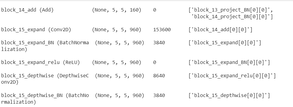
# Set the layers of the base model as non-trainable (freeze the weights)
base_model.trainable = False
# Print a summary of the architecture of the base model
base_model.summary()

# Create a GlobalAveragePooling2D layer to compute the average value of each feature map in the batch
global_average_layer = tf.keras.layers.GlobalAveragePooling2D()

# Apply global average pooling to the batch of image features
feature_batch_average = global_average_layer(feature_batch)

# Print the shape of the resulting pooled features
print(feature_batch_average.shape)

# Create a Dense layer for making predictions
prediction_layer = tf.keras.layers.Dense(1)

# Apply the Dense layer to the global average pooled features
# to generate prediction scores for each input image in the batch
prediction_batch = prediction_layer(feature_batch_average)

# Print the shape of the resulting prediction batch
print(prediction_batch.shape)

As we can observe, both the validation accuracy and the training accuracy have increased, which means model performance has increased for both the test set and the training set. Along with this, training and validation loss has decreased during training.

This shows that the model training has been successful using transfer learning. 

How to evaluate and test a transfer learning model

After splitting the dataset and choosing the pre-trained model, we can use the validation set to evaluate the model’s performance during training. Training measures that we can take involve measuring the accuracy, precision, recall, or F1 score of the model. We can also use visualization techniques like the confusion metric or ROC curves.

After evaluation, we can carry out fine-tuning the model and repeat the previous step. We can continue like this until we are satisfied with the model's performance. We can also try changing the hyperparameters of the model, or we can modify the architecture of the model to see if it increases the performance.

Examples of Transfer learning being used

Image recognition- Transfer learning has been proven to be successful in the Image recognition task. Pre-trained CNN models like VGG16 have been used for feature extraction to aid new models. These models have been used in various applications like object recognition, facial recognition, and in medical image analysis.

Natural Language Processing- Pre-trained models like BERT have also contributed to transfer learning in this domain. These models can be fine-tuned for various NLP tasks like text classification, sentiment analysis, etc

Speech Recognition- Transfer learning has been used in speech recognition to transfer knowledge learned from one language to another. For example, a pre-trained model trained on English speech can be fine-tuned for use in Spanish speech recognition, increasing its performance.

Some tips and Best Practices

We should choose a proper learning rate suitable for our specific task- We have to choose the pre-trained models according to the domain of our task and also the specific target of our classes. For example, using CNN models like ResNet for image recognition tasks.

Fine-tune - We should fine-tune our pre-trained models as it is far more efficient than training from scratch.

Freeze some layers of the pre-trained model- Freezing these layers can help preserve the knowledge learned in the pre-trained model and prevent overfitting.

Some pitfalls to avoid

Overfitting- If the model becomes too complex it can lead to overfitting problems, this can also arise if the training dataset needs to be bigger.

Underfitting- If the model needs to be fine-tuned enough, it can lead to the model being too complex to capture the complexity of the data. This can also happen if the dataset needs to be simplified.

In this article, we have discussed the fundamentals of transfer learning, how to prepare data for this purpose, how to build a base model, fine-tune the pre-trained models. Next, we applied transfer learning to a new dataset. Finally, we discussed how to evaluate a transfer-learning model, discussed some examples of transfer learning, some tips and practices, and some pitfalls to avoid.

Transfer learning can potentially change how learning takes place with specific datasets; it helps immensely in saving both time and resources in model training.

It is essential for anyone learning about deep learning what transfer learning is, as it is common practice to use transfer learning in almost every domain of deep learning.