Image Generation with DCGANs in Computer Vision | Computer Vision

Written by- AionlinecourseComputer Vision Tutorials

Have you ever wondered how computers can create pictures automatically, transform the image style, and make art like an artist? It’s a fascinating journey into the world, where pixels become the canvas, and algorithms wield the paintbrush to craft images that blur the line between human and machine creativity. The secret behind the technique is something called “GAN” that stands for Generative Adversarial Networks. Today, we will explore image generation methods with DCGANs. Stay tuned!!!

Before jumping the whole tutorial, let’s know what will be explored today.

Brief introduction of image generation
Discuss about the types of image generation techniques
Understanding the architecture of DCGANs
Developing a model
Challenges and necessary steps
Conclusion and Further Exploration

Image generation is a process in computer vision where computers are used to create visual images, transform images into one style to another, generate images from text and others. This technology uses neural networks to generate images that can be realistic and artistic. Generally this process learns to capture the underlying distribution of the training data and generate new data samples by following the learned distribution pattern.

Significance of Image Generation

It plays a significant role in various industries and increases creativity in those fields. Some examples are:

It aids fashion designers in creating unique clothing patterns, textures, textile designs and so on.
In healthcare, it generates synthetical medical images for training AI models that enhance diagnostic tools.
It increases the creativity of the artists to foster innovation in the world of art and design.
It helps to generate synthetic data that can be used as data augmentation technique.
It helps in the Entertainment and Gaming industries by enhancing graphics, special effects and character design in video games and animations.
Architects and interior designers use image generation to visualise architectural designs and interior spaces.
It can be used in anomaly detection and security.

Apart from these usage, image generation can be used in urban planning and architecture visualisation, virtual reality and augmented reality, research and development, education and so on.

Different types of image generation techniques

Image generation models are used to generate images either from scratch or by modifying existing images. There are several deep learning models for image generation techniques with their own unique approach and characteristics.

Autoencoder: It consists of an encoder and a decoder where the encoder compresses the input data into lower dimensional representations and the decoder reconstructs the input from lower dimensional representations.

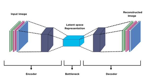
Several variations of autoencoder like denoising autoencoder can be used for image generation.

Variational Autoencoders (VAEs): It is a generative model that learns a probabilistic distribution of data. It is a variation of autoencoder that has the ability to generate new data samples by sampling from a continuous latent space.

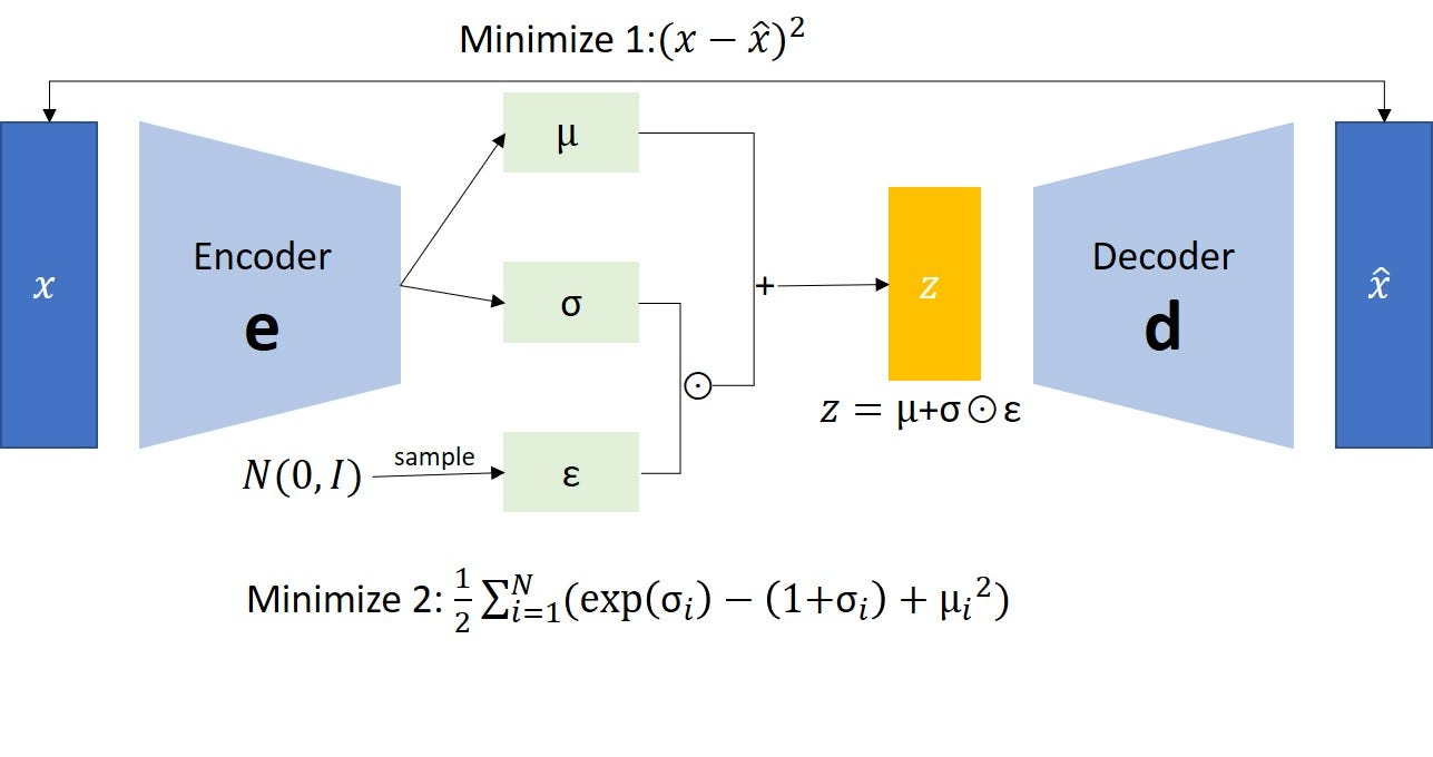
VAEs encode the high dimensional data to low dimensional latent space where the latent space is in probabilistic distribution. Then the decoder generates new data samples from the latent space. It can be used for image denoising, style transfer and many other image generation tasks.

Generative Adversarial Networks (GANs): It consists of two neural networks such as generator model and discriminator model. The generator network takes random noise as input and generates new data while the discriminator model is responsible for distinguishing whether the data is real or fake.

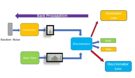
The aim of the generator model is to fool the discriminator by generating the data as real data. There are many variations of GANs already published. Today we will go through with the Deep Convolutional GAN (DCGAN) model.

There are many other algorithms like PixelRNN and PixelCNN, Deep Belief Networks, variation of GANs can be applied as image generation techniques.

Why is DCGAN needed over GAN?

Deep Convolutional Generative Adversarial Networks were introduced to address some of the limitations and challenges associated with the GAN. Original GAN has a possibility of mode collapse of the model. Mode collapse indicates a problem where the model always generates the same things where other things are being ignored. Suppose there are 10 different images but the model generates only 2/3 different images. This is mode collapse. DCGANs is designed to solve this issue. Then it is more stable during training than GANs. It has the ability to capture low level features and then build up more complex features. It can produce high quality images over GAN. That’s why DCGAN is needed over GAN.

DCGAN Architecture

It is a special configuration of GAN. It consists of a Generator and Discriminator model which work together in an adversarial network. DCGAN architecture follows the same GAN methodology, just changing some internal architecture. The changes are:

It converts max-pooling layers to convolutional layers
It converts fully connected layers to global average pooling layers in the discriminator model
It uses batch normalisation layers in both generator and discriminator model
It uses leaky relu activation function in the discriminator model

The DCGAN model uses convolutional layers without max pooling or fully connected layers. It uses convolutional stride for downsampling and transposed convolution for up sampling.

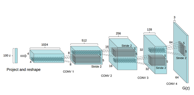
The Generator model takes a 100*1 noise vector using normal distribution as an input and maps it into 64*64*3. The network expends the random noise from 100*1 to 1024*4*4 size which is denoted as project and reshape. Then the model performed a fractionally strided convolution 4 times with a stride of ½ that means every time of applying, it will double the image dimension while reducing the number of output channels. That’s why, we see the network size goes from:

100*1 > 1024*4*4 > 512*8*8 > 256*16*16 > 128*32*32 > 64*64*3

So, the dimensions of the generated output is (64*64*3).

The aim of the Discriminator model is to determine if the images are real or fake. It is designed similar to the Convolutional Neural Network to perform a binary image classification task. Although the author of the paper suggested some changes like using only strided convolution with LeakyRelu activation function instead of using fully connected layers. Use batch Normalisation except the output and input layer of the discriminator model.

Overall DCGAN model indicates replacing all max pooling layer with convolutional stride, using transpose convolution for upsampling, eliminate all fully connected layers, using batch normalisation in the generator and discriminator model except input and output layer, using Relu activation in the generator model and for the output which uses tanh, and LeakyRelu activation can be used in discriminator.

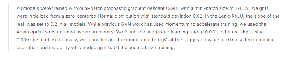
For tuning the DCGAN model, this is taken directly from the paper.

Hope, you can understand the image generation techniques and the architecture of the DCGAN model. Let’s solve a real world problem with the DCGAN model.

Problem domain

We want to generate the Celebrity faces from the DCGAN model. For training the model, we will use the Celeb-A Faces dataset or take the dataset from here. Let’s get started.

Implementation of DCGAN model

First import the necessary libraries to load the data, preprocess data, create DCGAN model, train the model and evaluate. You will get the full project code on Google Colab. We will use the pytorch framework for deep learning models. The “argparse” is for command line argument parsing, and numpy, os, matplotlib is for data preprocessing and data visualisation.

#%matplotlib inline
import argparse
import os
import random
import torch
import torch.nn as nn
import torch.nn.parallel
import torch.optim as optim
import torch.utils.data
import torchvision.datasets as dset
import torchvision.transforms as transforms
import torchvision.utils as vutils
import numpy as np
import matplotlib.pyplot as plt
import matplotlib.animation as animation
from IPython.display import HTML

# Set random seed for reproducibility
manualSeed = 999
#manualSeed = random.randint(1, 10000) # use if you want new results
print("Random Seed: ", manualSeed)
random.seed(manualSeed)
torch.manual_seed(manualSeed)
torch.use_deterministic_algorithms(True) # Needed for reproducible results

Random Seed: 999

The code is responsible for setting up various hyperparameters and configuration options for training a DCGAN model. These parameters will be utilised at the time of training the model.

# Root directory for dataset
dataroot = "Path of the data folder"
# Number of workers for dataloader
workers = 2
# Batch size during training
batch_size = 128
# Spatial size of training images. All images will be resized to this
#   size using a transformer.
image_size = 64
# Number of channels in the training images. For color images this is 3
nc = 3
# Size of z latent vector (i.e. size of generator input)
nz = 100
# Size of feature maps in generator
ngf = 64
# Size of feature maps in discriminator
ndf = 64
# Number of training epochs
num_epochs = 5
# Learning rate for optimizers
lr = 0.0002
# Beta1 hyperparameter for Adam optimizers
beta1 = 0.5
# Number of GPUs available. Use 0 for CPU mode.
ngpu = 1

Create Dataset & prepare data for training

Create the dataset from the image data folder where we use some transformation of images like resizing into the image size, centre cropping,convert the image into a tensor array and then normalise the tensor. Then create a data loader to convert the data into batch size and efficient training in the model. Then define the device as a CPU or GPU. Then take a batch of images from the data loader and show the images.

# We can use an image folder dataset the way we have it setup.
# Create the dataset
dataset = dset.ImageFolder(root=dataroot,
                           transform=transforms.Compose([
                               transforms.Resize(image_size),
                               transforms.CenterCrop(image_size),
                               transforms.ToTensor(),
                               transforms.Normalize((0.5, 0.5, 0.5), (0.5, 0.5, 0.5)),
                           ]))
# Create the dataloader
dataloader = torch.utils.data.DataLoader(dataset, batch_size=batch_size,
                                         shuffle=True, num_workers=workers)
# Decide which device we want to run on
device = torch.device("cuda:0" if (torch.cuda.is_available() and ngpu > 0) else "cpu")
# Plot some training images
real_batch = next(iter(dataloader))
plt.figure(figsize=(8,8))
plt.axis("off")
plt.title("Training Images")
plt.imshow(np.transpose(vutils.make_grid(real_batch[0].to(device)[:64], padding=2, normalize=True).cpu(),(1,2,0)))

Our dataset is ready for training. Let’s start the model creation part. First it is needed to initialise the weights and biases of the model. For convolutional layers, we initialise the weights with normal distribution(mean 0 and standard deviation 0.02). For batch normalisation layers, it initialises the weights from normal distribution with mean 1 and standard deviation 0.02 and the biases with a value of 0.

# custom weights initialization called on ``netG`` and ``netD``
def weights_init(m):
    # extract the class name of the layer
    classname = m.__class__.__name__
    if classname.find('Conv') != -1:
        nn.init.normal_(m.weight.data, 0.0, 0.02)
    elif classname.find('BatchNorm') != -1:
        nn.init.normal_(m.weight.data, 1.0, 0.02)
        nn.init.constant_(m.bias.data, 0)

Generator Model

The generator model is responsible for creating synthetic images that resemble real images. Here self.main is the generator architecture that consists of several transposed convolutional layers which are used to upsample the input noise vector and transform it into an image. ‘ngpu’ indicates the number of GPU, ‘nz’ is for number of channels in the input noise vector, ‘ngf * 8’ indicates the number of output channels where ‘ngf’ is for the number of feature maps, and ‘nc’ indicates the number of channels of the image.

Overall, it takes a noise vector as input and uses a series of transposed convolutional layers with batch normalisation and ReLU activations to transform the noise into a synthetic image that mimics real images.

# Generator Code
class Generator(nn.Module):
    def __init__(self, ngpu):
        super(Generator, self).__init__()
        self.ngpu = ngpu
        self.main = nn.Sequential(
            # input is Z, going into a convolution
		# nz=input, ngf*8=output, 4= kernel size, 1=stride, 0=padding
            nn.ConvTranspose2d( nz, ngf * 8, 4, 1, 0, bias=False),
		# batch norm normalize the output of convolutional layer
            nn.BatchNorm2d(ngf * 8),
            nn.ReLU(True),
            # state size. ``(ngf*8) x 4 x 4``
            nn.ConvTranspose2d(ngf * 8, ngf * 4, 4, 2, 1, bias=False),
            nn.BatchNorm2d(ngf * 4),
            nn.ReLU(True),
            # state size. ``(ngf*4) x 8 x 8``
            nn.ConvTranspose2d( ngf * 4, ngf * 2, 4, 2, 1, bias=False),
            nn.BatchNorm2d(ngf * 2),
            nn.ReLU(True),
            # state size. ``(ngf*2) x 16 x 16``
            nn.ConvTranspose2d( ngf * 2, ngf, 4, 2, 1, bias=False),
            nn.BatchNorm2d(ngf),
            nn.ReLU(True),
            # state size. ``(ngf) x 32 x 32``
            nn.ConvTranspose2d( ngf, nc, 4, 2, 1, bias=False),
            nn.Tanh()
            # state size. ``(nc) x 64 x 64``
        )
    def forward(self, input):
        return self.main(input)

The code creates the generator model of DCGAN as netG, handles multi-GPU training if you configured, initialised the model’s weight and print the summary of the model.

# Create the generator
netG = Generator(ngpu).to(device)
# Handle multi-GPU if desired
if (device.type == 'cuda') and (ngpu > 1):
    netG = nn.DataParallel(netG, list(range(ngpu)))
# Apply the ``weights_init`` function to randomly initialize all weights
#  to ``mean=0``, ``stdev=0.02``.
netG.apply(weights_init)
# Print the model
print(netG)

Generator( (main): Sequential( (0): ConvTranspose2d(100, 512, kernel_size=(4, 4), stride=(1, 1), bias=False) 
(1): BatchNorm2d(512, eps=1e-05, momentum=0.1, affine=True, track_running_stats=True) 
(2): ReLU(inplace=True) 
(3): ConvTranspose2d(512, 256, kernel_size=(4, 4), stride=(2, 2), padding=(1, 1), bias=False) 
(4): BatchNorm2d(256, eps=1e-05, momentum=0.1, affine=True, track_running_stats=True) 
(5): ReLU(inplace=True) 
(6): ConvTranspose2d(256, 128, kernel_size=(4, 4), stride=(2, 2), padding=(1, 1), bias=False) 
(7): BatchNorm2d(128, eps=1e-05, momentum=0.1, affine=True, track_running_stats=True) 
(8): ReLU(inplace=True) 
(9): ConvTranspose2d(128, 64, kernel_size=(4, 4), stride=(2, 2), padding=(1, 1), bias=False) 
(10): BatchNorm2d(64, eps=1e-05, momentum=0.1, affine=True, track_running_stats=True) 
(11): ReLU(inplace=True) 
(12): ConvTranspose2d(64, 3, kernel_size=(4, 4), stride=(2, 2), padding=(1, 1), bias=False) 
(13): Tanh() ) )

Discriminator Model

This is the Discriminator network for DCGAN which consists of several convolutional layers with Leaky ReLU activations. It is just a classification model that identifies whether the input image is real or fake. The argument ‘ngpu’ indicates the number of GPUs to be used. ‘Ndf’ is for feature maps and ‘nc’ indicates the channels of the images. ‘Sigmoid’ activation function is used in the output layer because of binary classification. The network produces a probability score indicating whether the input image is real or fake.

class Discriminator(nn.Module):
    def __init__(self, ngpu):
        super(Discriminator, self).__init__()
        self.ngpu = ngpu
        self.main = nn.Sequential(
            # input is ``(nc) x 64 x 64``
            nn.Conv2d(nc, ndf, 4, 2, 1, bias=False),
            nn.LeakyReLU(0.2, inplace=True),
            # state size. ``(ndf) x 32 x 32``
            nn.Conv2d(ndf, ndf * 2, 4, 2, 1, bias=False),
            nn.BatchNorm2d(ndf * 2),
            nn.LeakyReLU(0.2, inplace=True),
            # state size. ``(ndf*2) x 16 x 16``
            nn.Conv2d(ndf * 2, ndf * 4, 4, 2, 1, bias=False),
            nn.BatchNorm2d(ndf * 4),
            nn.LeakyReLU(0.2, inplace=True),
            # state size. ``(ndf*4) x 8 x 8``
            nn.Conv2d(ndf * 4, ndf * 8, 4, 2, 1, bias=False),
            nn.BatchNorm2d(ndf * 8),
            nn.LeakyReLU(0.2, inplace=True),
            # state size. ``(ndf*8) x 4 x 4``
            nn.Conv2d(ndf * 8, 1, 4, 1, 0, bias=False),
            nn.Sigmoid()
        )
    def forward(self, input):
        return self.main(input)

Now create the discriminator model (‘netD’) for the DCGAN, handle multi-GPU support, applies weight initialization and print the model.

# Create the Discriminator
netD = Discriminator(ngpu).to(device)
# Handle multi-GPU if desired
if (device.type == 'cuda') and (ngpu > 1):
    netD = nn.DataParallel(netD, list(range(ngpu)))
# Apply the ``weights_init`` function to randomly initialize all weights
# like this: ``to mean=0, stdev=0.2``.
netD.apply(weights_init)
# Print the model
print(netD)

Discriminator( (main): Sequential( (0): Conv2d(3, 64, kernel_size=(4, 4), stride=(2, 2), padding=(1, 1), bias=False) 
(1): LeakyReLU(negative_slope=0.2, inplace=True) 
(2): Conv2d(64, 128, kernel_size=(4, 4), stride=(2, 2), padding=(1, 1), bias=False) 
(3): BatchNorm2d(128, eps=1e-05, momentum=0.1, affine=True, track_running_stats=True) 
(4): LeakyReLU(negative_slope=0.2, inplace=True) 
(5): Conv2d(128, 256, kernel_size=(4, 4), stride=(2, 2), padding=(1, 1), bias=False) 
(6): BatchNorm2d(256, eps=1e-05, momentum=0.1, affine=True, track_running_stats=True) 
(7): LeakyReLU(negative_slope=0.2, inplace=True) 
(8): Conv2d(256, 512, kernel_size=(4, 4), stride=(2, 2), padding=(1, 1), bias=False) 
(9): BatchNorm2d(512, eps=1e-05, momentum=0.1, affine=True, track_running_stats=True) 
(10): LeakyReLU(negative_slope=0.2, inplace=True) 
(11): Conv2d(512, 1, kernel_size=(4, 4), stride=(1, 1), bias=False) (12): Sigmoid() 
) )

Now prepare the loss function as binary cross entropy loss (‘BCELoss’) that calculates the error between the discriminator’s output and the ground truth. Then create a fixed batch of latent vectors for visualisation. Then create optimizers for the generator and discriminator model for training the DCGAN.

# Initialize the ``BCELoss`` function
criterion = nn.BCELoss()
# Create batch of latent vectors that we will use to visualize
#  the progression of the generator
fixed_noise = torch.randn(64, nz, 1, 1, device=device)
# Establish convention for real and fake labels during training
real_label = 1.
fake_label = 0.
# Setup Adam optimizers for both G and D
optimizerD = optim.Adam(netD.parameters(), lr=lr, betas=(beta1, 0.999))
optimizerG = optim.Adam(netG.parameters(), lr=lr, betas=(beta1, 0.999))

We have created the generator and discriminator model. Then setting up all the parameters to train the model. Now we are ready to train. So the following code trains the DCGAN model by iteratively updating the discriminator and generator networks weights. The model tries to minimise the discriminator’s error on real and fake data and maximises the generator’s ability to produce fake data that is classified as real by the discriminator. The training processes for a specified number of epochs. The losses and generated images are saved for visualisation and analysis.

# Training Loop
# Lists to keep track of progress
img_list = []
G_losses = []
D_losses = []
iters = 0
print("Starting Training Loop...")
# For each epoch
for epoch in range(num_epochs):
    # For each batch in the dataloader
    for i, data in enumerate(dataloader, 0):
        ############################
        # (1) Update D network: maximize log(D(x)) + log(1 - D(G(z)))
        ###########################
        ## Train with all-real batch
        netD.zero_grad()
        # Format batch
        real_cpu = data[0].to(device)
        b_size = real_cpu.size(0)
        label = torch.full((b_size,), real_label, dtype=torch.float, device=device)
        # Forward pass real batch through D
        output = netD(real_cpu).view(-1)
        # Calculate loss on all-real batch
        errD_real = criterion(output, label)
        # Calculate gradients for D in backward pass
        errD_real.backward()
        D_x = output.mean().item()
        ## Train with all-fake batch
        # Generate batch of latent vectors
        noise = torch.randn(b_size, nz, 1, 1, device=device)
        # Generate fake image batch with G
        fake = netG(noise)
        label.fill_(fake_label)
        # Classify all fake batch with D
        output = netD(fake.detach()).view(-1)
        # Calculate D's loss on the all-fake batch
        errD_fake = criterion(output, label)
        # Calculate the gradients for this batch, accumulated (summed) with previous gradients
        errD_fake.backward()
        D_G_z1 = output.mean().item()
        # Compute error of D as sum over the fake and the real batches
        errD = errD_real + errD_fake
        # Update D
        optimizerD.step()
        ############################
        # (2) Update G network: maximize log(D(G(z)))
        ###########################
        netG.zero_grad()
        label.fill_(real_label)  # fake labels are real for generator cost
        # Since we just updated D, perform another forward pass of all-fake batch through D
        output = netD(fake).view(-1)
        # Calculate G's loss based on this output
        errG = criterion(output, label)
        # Calculate gradients for G
        errG.backward()
        D_G_z2 = output.mean().item()
        # Update G
        optimizerG.step()
        # Output training stats
        if i % 50 == 0:
            print('[%d/%d][%d/%d]\tLoss_D: %.4f\tLoss_G: %.4f\tD(x): %.4f\tD(G(z)): %.4f / %.4f'
                  % (epoch, num_epochs, i, len(dataloader),
                     errD.item(), errG.item(), D_x, D_G_z1, D_G_z2))
        # Save Losses for plotting later
        G_losses.append(errG.item())
        D_losses.append(errD.item())
        # Check how the generator is doing by saving G's output on fixed_noise
        if (iters % 500 == 0) or ((epoch == num_epochs-1) and (i == len(dataloader)-1)):
            with torch.no_grad():
                fake = netG(fixed_noise).detach().cpu()
            img_list.append(vutils.make_grid(fake, padding=2, normalize=True))
        iters += 1

Starting Training Loop... 
[0/5][0/1583]	Loss_D: 1.8962	Loss_G: 5.3561	D(x): 0.5589	D(G(z)): 0.6206 / 0.0083 
[0/5][50/1583]	Loss_D: 0.1939	Loss_G: 9.4058	D(x): 0.9158	D(G(z)): 0.0347 / 0.0002
—--------------------------------------------------
[4/5][1500/1583]	Loss_D: 0.6967	Loss_G: 1.7715	D(x): 0.6409	D(G(z)): 0.1639 / 0.2021
[4/5][1550/1583]	Loss_D: 0.4795	Loss_G: 2.6125	D(x): 0.8206	D(G(z)): 0.2225 / 0.0910

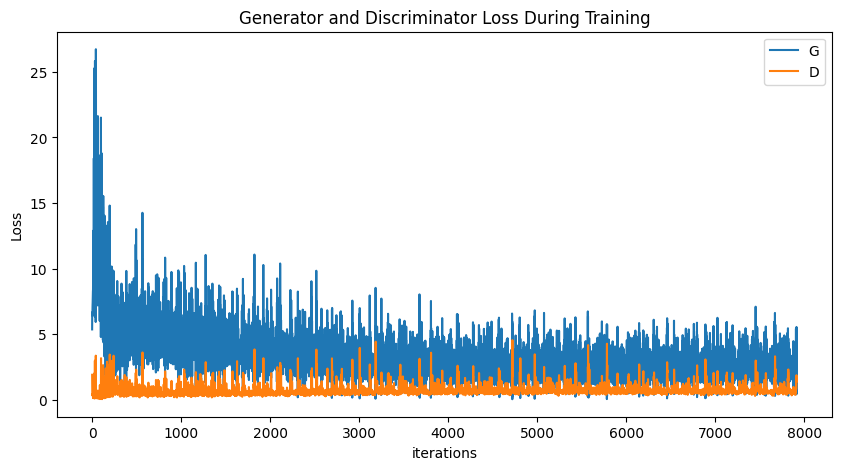
Let’s visualise the generator and discriminator losses during training. This visualisation helps you to monitor whether the generator loss decreases and approaches zero while the discriminator loss decreases as well. So, we can tell that the generator is becoming better at generating realistic images.

plt.figure(figsize=(10,5))
plt.title("Generator and Discriminator Loss During Training")
plt.plot(G_losses,label="G")
plt.plot(D_losses,label="D")
plt.xlabel("iterations")
plt.ylabel("Loss")
plt.legend()
plt.show()

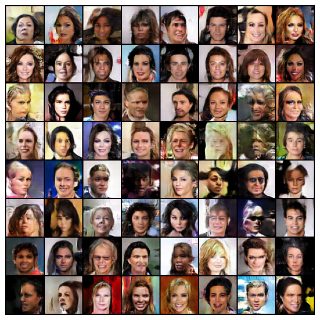
We can generate an animation to visualise the progression of the generator’s output during training by the following code. This animation is super helpful to visualise how the quality of generated images improves over time as the generator network and becomes better at generating realistic images. When you run the code, you will see the animation bar in your notebook. Here we just plot some generated images which are produced by the generator model during training at the last epoch.

fig = plt.figure(figsize=(8,8))
plt.axis("off")
ims = [[plt.imshow(np.transpose(i,(1,2,0)), animated=True)] for i in img_list]
ani = animation.ArtistAnimation(fig, ims, interval=1000, repeat_delay=1000, blit=True)
HTML(ani.to_jshtml())

Now the trained generator model can generate images as real data. So take a batch of real images and generate a number of images. Then compare the real images and generated images.

# Grab a batch of real images from the data loader
real_batch = next(iter(dataloader))
# Plot the real images
plt.figure(figsize=(15,15))
plt.subplot(1,2,1)
plt.axis("off")
plt.title("Real Images")
plt.imshow(np.transpose(vutils.make_grid(real_batch[0].to(device)[:64], padding=5, normalize=True).cpu(),(1,2,0)))
# Plot the fake images from the last epoch
plt.subplot(1,2,2)
plt.axis("off")
plt.title("Fake Images")
plt.imshow(np.transpose(img_list[-1],(1,2,0)))
plt.show()

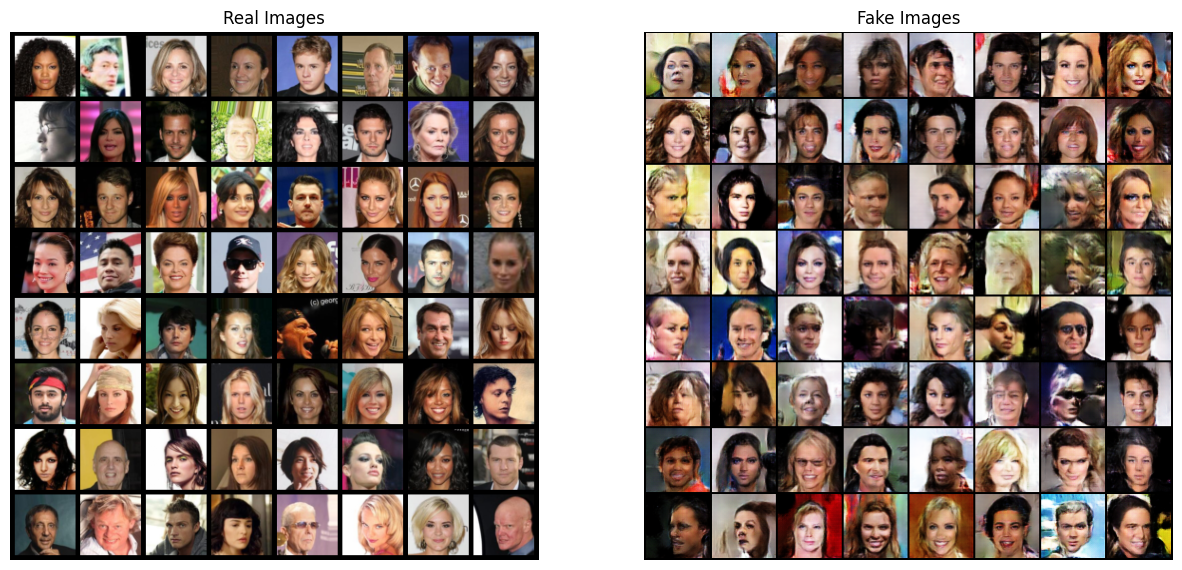
Great. We have implemented the DCGAN model and generated images by the generator model.

Evaluating Generated Images

Evaluating the quality of generated images is a crucial step in assessing the performance of generative models. There are several qualitative and quantitative metrics that can be employed to evaluate the generated images.

Qualitative Evaluation: Visual Inspection, Domain Expert Review, User Feedback can be used to evaluate the generated images. Human evaluators can judge the quality, realism and diversity of the generated content. Domain experts or artists can review the generated images to assess their quality. In the real world applications, user feedback can be valuable.

Quantitative Evaluation: There are some metrics that can measure the quality of the generated images such as:

Inception Score(IS): It evaluates the quality and diversity of the generated images. It measures how well the generated images can be classified by an Inception v3 model where higher IS values indicate better image quality and diversity.
Frechet Inception Distance (FID): It measures the similarity between real and generated images where lower FID values indicate better image quality and diversity.
Structural Similarity Index (SSIM): It measures the structural similarity between generated and real images. Higher SSIM values indicate better quality.

There are other quantitative evaluations like Peak Signal to Noise Ratio (PSNR), Total Variation(TV) Loss and others. The choice of evaluation metrics should align with the goals and requirements of the specific use case. A single metric can’t provide complete evaluation of generated images. So, A combination of qualitative and quantitative methods can be a more robust approach for evaluation.

Challenges in Image Generation

DCGANs have made significant progress in image generation but it faces some challenges during training and evaluation such as:

Mode Collapse: It occurs when the generator produces similar types of images and fails to capture full diversity of the data. Modifying loss function, adjusting network architecture can be taken to solve the issue.
Vanishing Gradients: During training, gradients can become too small and lead to slow convergence. Weight initialization, different activation functions can be used to mitigate the issue.
Training Unstability: It is challenging to stabilise during training. Different variants of GANs can be used in this issue.
Hyperparameter Tuning: Setting the perfect hyperparameters like learning rate, batch size, weight initialization and others are important for successful training.
Overfitting: It may occur when the generator model memorises the training data instead of learning to generate a new, diverse image. To overcome, use regularisation, dropout, early stopping or other methods.

At the time of experimenting with DCGAN, we can face these types of problems. So, use different variants of GANs or fix the specific issue during training. The researchers are continuously working to improve training stability, quality and efficiency of the model.

Balancing exploration and exploitation

Exploitation involves the generation model producing samples that are highly similar to the training data. It is about making the most of the knowledge gained from the training data to generate images that closely resemble the data distribution.

Exploration involves the generative model producing samples that are different from the training data. It aims to produce novel and diverse images that may not be present in the training dataset.

Balancing the exploitation and exploration is a crucial task. Where overemphasise exploitation may lead to mode collapse and produce the same or similar samples. On the other hand, excessive exploration may result in unrealistic and poor quality samples. So the goal of DCGAN is to strike the right balance between exploration and exploitation so that the generator can produce high quality and diverse images that are both realistic and novel.

Recent advancements and future research directions

It has been widely used in many applications including image generation, image editing, image to image translation and many others. Some of the recent works on DCGANs are given below.

Transfer learning techniques have been applied to DCGANs so that it can improve its performance and generate high quality images.
It has been used in medical image analysis such as segmentation, registration, classification and others.
Researchers have introduced more improved architectures like PCGAN to generate high resolution images.
To stabilise and converge speed of DCGAN, the researchers had introduced WGAN and others.
It has been used in image to image translation, improved video generation, improved text to image synthesis, improved image editing and so on. Actually the applications of DCGANs are growing day by day.

Model Deployment

First train the DCGAN model with a dataset. Then convert the trained model to a suitable format for deployment if needed like ONNX or others. Then deploy the model in a suitable platform. It can be a local server, cloud based platform, Android/ios, web framework, or even an edge device like Raspberry Pi or others. It is needed to remember that deploying models in a production environment requires careful consideration of factors like scalability, maintainability and security. It is also important to monitor the model’s performance over time and retrain it as needed with new data.

Conclusion and further exploration

In this tutorial, we have discussed the concept of the image generation, significance and applications of image generation, and discussed various image generation techniques like autoencoders, variational autoencoders, and GANs. Then we discussed the architecture of DCGAN and implemented a problem. Then discuss the evaluation techniques, some recent advancements, challenges and deployment strategy. Hope this discussion gives you an overall idea of image generation.

As further exploration of image generation, we can forward to more complex architectures of GANs and can be applied in various applications. As well as image generation, we can use it in video generation and others. The research is going on and I will keep calm with the updates. Dive deeper, experiment, and uncover the full capabilities of generative models in pushing the boundaries of artificial creativity.

Previous Next