A Comprehensive Guide to Image Segmentation in Computer Vision | Computer Vision

Today’s world is filled with pictures where every photo holds a story. Have you ever thought about how self-driving cars understand the road so well? How a machine can accurately tell about the disease by just getting a picture of the organs. How can a machine automatically track any objects and analyse them? How do sports organisations monitor the game rules accurately and perform analysis for better situations? The secret behind these feats is something called ‘Image Segmentation’. Today we will explore all the parts of Image Segmentation. Let’s dive in.

Let’s know what we are going to explore in this article before jumping into the whole tutorial. 

• Brief introduction of Image Segmentation
• Discuss about the types of Image Segmentation
• Various methods of Image Segmentation
• Solution of real world Image Segmentation problem
• Model Deployment and real world usage
• Challenges
• Conclusion and future directions

Image Segmentation is a fundamental concept of Computer Vision that segments the different objects in an image or video frame. This technology focuses on enabling computers to understand and interpret visual information from images. It is a process of dividing an image into meaningful and distinct regions or segments where each region represents a specific object, or feature of the image. In simple terms, Image Segmentation defines the region of any object in the image that can be processed or analysed for further work. 

Importance of Image Segmentation

Image segmentation is the process of breaking down images into meaningful components that contains a lot of significant in the wide range of applications across various industries and technologies such as:

• It identifies and isolates different elements or objects within an image that is highly needed in medical image analysis or autonomous driving technique.
• It can pinpoint exact location and boundaries of objects that makes it easier to recognize and analyse them.
• It helps to extract the specific features and attributes within an image that can be used in facial recognition where eyes, nose, mouth can be identified.
• It helps to understand the content and context of an image.
• It can help to track objects in video analysis that can be performed in surveillance, autonomous vehicles, sports analysis, health conditions and so on.

Overall, its significance lies in enabling computers to recognize objects, understand image content and context, track movement and make informed decisions from images and videos.

Applications of Image Segmentation

Hope, you realise the significance of image segmentation. Now let’s understand the area where we can apply this technique to make our life easier. It has plenty of applications. Among them, some popular ones are discussed below.

• Autonomous Vehicles: It can be used in road object detection(pedestrians,vehicles, traffic signs etc), lane detection( identify lane markings and maintain proper vehicle positioning) and so on.
• Security and Surveillance: It helps to identify unauthorised intruders and analyse moving objects.
• Agriculture: We can monitor crop health, detect diseases, optimising farming practices by applying image segmentation on satellite and drone images.
• Robotics: It assists robots in understanding the surroundings to navigate and avoid obstacles.
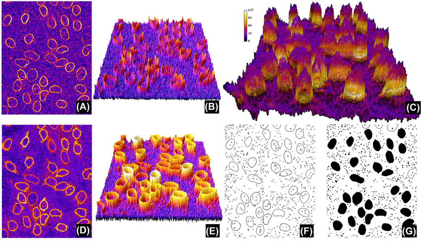
• Medical Imaging: It is highly used in medical science such as Tumour Detection, Organ Segmentation, Cell Analysis and so on.
• Geographic Information Systems: By aerial and satellite image segmentation, we can analyse our land accurately so that it can be used in urban planning, environmental monitoring and so on.
• Quality Control and Manufacturing: It assists to identify defects in manufacturing processes and used to analyse materials for quality control.

Truely. It is an incredibly versatile and widely applicable concept and growing day by day. We can use this technique in object tracking and image editing, Augmented Reality, Disaster Management, Video Games, Gesture Recognition, Forensic Analysis, Biometrics, Traffic management, Human Pose Estimation and so many other fields. Hope, you can understand the significance and applicable area of image segmentation. Let’s go deep.

Types of Image Segmentation

There are mainly two types of image segmentation that are traditional image segmentation and deep learning based image segmentation. Traditional image segmentation refers to the process of segmenting an object from image through a group of image analysis techniques. These methods depend  on various principles and algorithms to partition an image into distinct regions or segments based on certain criteria. These methods are Thresholding, Edge Based Segmentation, Region Based Segmentation, Clustering Based, Graph Based Segmentation and so on. 

Let’s learn all the methods briefly.

• Threshold Based Segmentation: This is the simplest method that selects a pixel intensity value as a threshold and classifies all pixels with intensities above or below the threshold into separate segments. Thresholding can be fixed or dynamic. A constant value is chosen in the fixed thresholding and adaptive methods can determine the threshold based on the image statistics in the dynamic threshold. This technique is computationally efficient and well suited for binary segmentation.

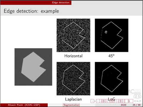
• Edge based segmentation: This technique focuses on detecting and representing the boundaries or edges of objects within an image. It identifies points in an image where there are significant changes in pixel values. Some edge detection operators are Sobel, Prewitt, Canny edge detectors and others. But it can be sensitive to noise and may produce spurious edges in noisy images. 

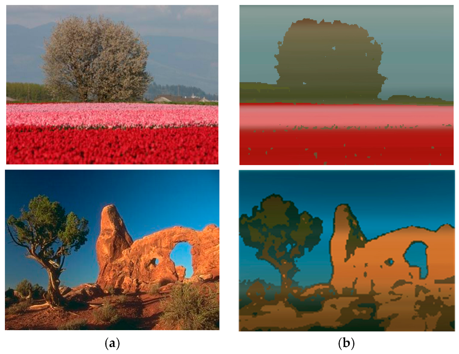
• Region based segmentation: It is another segmentation technique that aims to divide an image into meaningful regions or segments based on similarities in pixel properties such as colour, intercity, texture or other features. The goal is to group together pixels that belong to the same object or region in the image.  Here each region is made by a group of pixels and the algorithm locates via a seed point. 

• Clustering based segmentation: It is unsupervised algorithms that involves grouping similar pixels or regions in an image into clusters based on certain similarity criteria. The clustering algorithms are used to partition the image data into distinct segments or regions based on pixels in the image. K Means Clustering, Mean Shift Clustering, DBSCAN, Agglomerative Hierarchical Clustering, Fuzzy C Means are some methods of clustering based segmentation. Overall, It is a popular traditional problem for image segmentation.

• Graph based segmentation: It represents an image as a graph where pixels are nodes and edges connect nodes based on some measure of similarity or dissimilarity. The goal is to partition the graph into disjoint segments or regions while preserving meaningful image structures. It can capture the structural relationships between pixels. 

Deep Learning Based Segmentation is a modern and highly effective approach where the process of segment objects is developed by deep neural networks. These methods gives a remarkable accuracy to segment complex and varied images. In This process, there are mainly three types of segmentation such as semantic segmentation, instance segmentation and panoptic segmentation. 

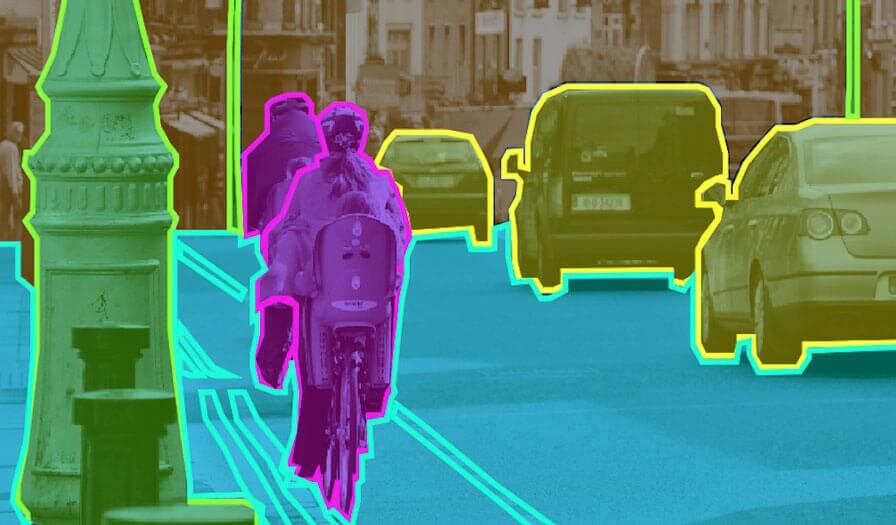
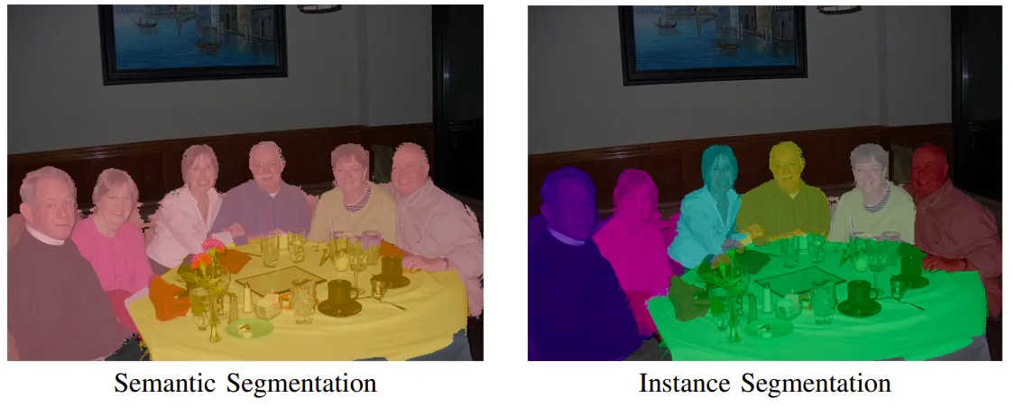
• Semantic Segmentation: This technique involves classifying each pixel in an image into several predefined categories. Here the pixels refer to a specific class and don’t provide any information or context. In the following picture, there are 2 people, 3 cars and others. This method defines all the persons as the only person category and 3 different cars are only defined as cars. 

There are various deep learning models that have been developed to perform semantic segmentation such as Fully Convolutional Networks(FCN), U-Net, SegNet, DeepLab, ENet and others. Semantic segmentation provides fine grained information about the contents of an image that is used in autonomous vehicles, medical images, object tracking, and others. Also, It leads to significant improvements in the accuracy and efficiency of the semantic segmentation models. 

• Instance Segmentation: Object detection and semantic segmentation combinedly creates instance segmentation. The goal is to identify individual objects or instances within an image. This means that different objects of the same class are distinguished as separate entities, even if they are the same category. 

There are many popular methods for instance segmentation such as Mask R-CNN, SOLO, Yolo and its variants, DETR and so on. This method is necessary in autonomous vehicles, Medical Image Analysis, Robotics, Augmented Reality and others. Instance segmentation provides a pixel wise understanding of objects in an image that makes it a more detailed and challenging task compared to semantic segmentation. 

• Panoptic Segmentation: It is a computer vision task that combines both instance segmentation and semantic segmentation to provide a comprehensive understanding of an image or a scene. The goal is to label and segment all image pixels into meaningful categories and also identify individual instances of each class. This technique is used in autonomous driving, object tracking, augmented reality & virtual reality, environment monitoring, scene understanding, and others.

Several models and approaches have been developed to address panoptic segmentation such as Panoptic FPN(Panoptic Feature Pyramid Network), UPSNet(Unified Panoptic Segmentation Network), Panoptic DeepLab, BlendMask, OneFormer, Mask DINO and others. 

Already we have learned about the various methods of image segmentation. The techniques are developing day by day. All the techniques are not possible to discuss. Today we will solve a real world problem of semantic segmentation with the help of the UNet model.

Data Preparation for Segmentation

Before training the segmentation model, it is highly needed to prepare the data label by pixel level annotations. Pixel level annotations indicate assigning each pixel in an image to a specific class or label. It provides precise information about the content of each pixel in an image and offers fine grained detail by labelling each pixel. It provides semantic information about the content of each pixel that allows the model to distinguish different object classes. It serves as a ground truth label for measuring accuracy, precision, recall, IoU and others.  The models(UNet, Mask R-CNN) learn each pixel with the correct class or object of image during training. Overall, they provide detailed and precise information about the exact boundaries and regions of interest within an image.

The process of creating ground truth masks

With the help of annotation software or tools, we can perform pixel wise annotation and create the label of the data. There are many annotation tools such as CVAT, Make Sense, Labelbox, Roboflow Annotate, labelMe, Labelimg, Label Studio, v7, encord annotate and others. 

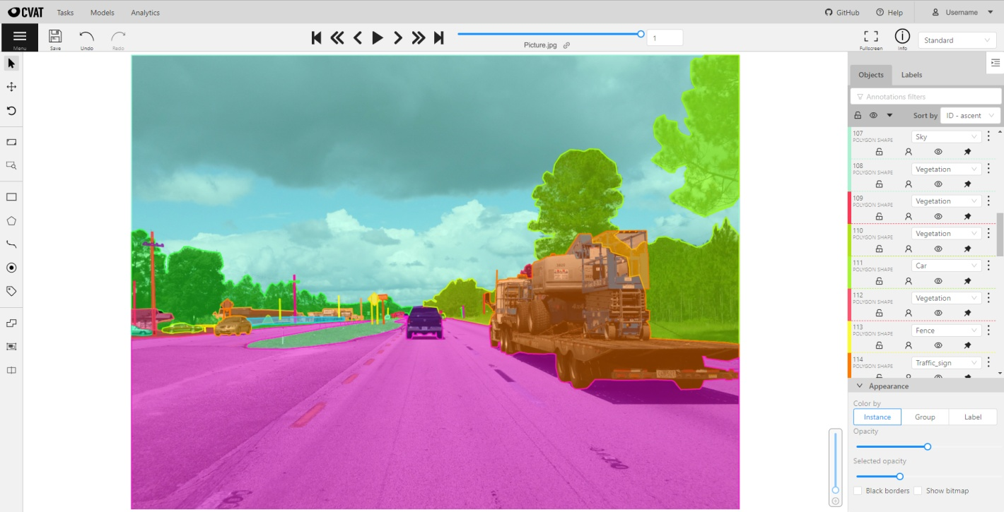
For annotation, first load the images you want to annotate to the annotation tool. Define the label of classes within the annotation software. Begin the annotation process by selecting an image to annotate, draw and outline the regions(polygons) of the objects in the image. Assign the corresponding class label to each annotated region based on the defined object classes. Pixel level annotation involves labelling each pixel within the annotated regions. Review the annotations to ensure that they accurately outline the regions or objects of interest. Then save the annotations as separate mask images for each input image. The annotated file will be considered as the label during training and evaluation. Now the images and labels are ready for further work.

Strategies for augmenting segmentation data

Augmenting segmentation data is a valuable strategy to enhance the diversity and quantity of the training images and labels for better model generalisation and performance. There are some libraries available to perform this task such as imgaug, albumentations, augmentor and others. There are several strategies for augmenting segmentation data are given below. 

• Apply Geometric transformations (rotation, scaling, flipping,translation and others) to images and corresponding masks.
• Randomly crop or pad images and masks to different sizes.
• Modify the colour and brightness of images in lighting conditions.
• Add random noise, apply blurring and sharpening filters to images and masks.
• Combine multiple images and masks to create composite images and corresponding masks. 

There are many other ways to perform augmentation in segmentation data but it is noted that over augmentation or aggressive augmentations can lead to unrealistic or noisy data which may negatively impact model performance. 

Problem Domain

Today we will solve a semantic segmentation problem using a popular kaggle dataset. This is an aerial semantic drone dataset that contains high resolution size(6000 * 4000px). The training set has 400 available images and corresponding masks. This is a multi-class problem that contains 23 classes. Because of semantic segmentation problems, we can use Fully Convolutional Network(FCN), U-Net, DeepLab and its variants, Yolo and its variants and other models. Any of them, we can choose. That’s why we will implement the problem with the U-Net model that is built upon the FCN model and modified in a way for better segmentation. 

U-Net Architecture

Olaf Ronneberger developed the UNet model for Bio Medical Image Segmentation where the architecture contains two paths (contraction path & symmetric expanding path). 

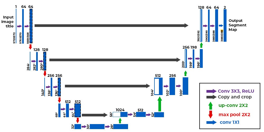
Contraction path also known as encoder, that is used to capture the context of the image. It is just like a CNN model (convolutional, max pooling, batch normalisation layers etc). The encoders are used to reduce the spatial dimensions of the feature maps and capture the features of the image. 

Bottleneck (Bridge) is one more convolutional layer before the decoder starts. It acts as a bridge between the encoder and decoder.

Symmetric Expanding path also known as decoder that uses transpose convolutional layers to increase the spatial resolution of the feature maps. These layers upsample the feature maps and allow the network to generate a pixel wise segmentation mask. The goal is to refine and segment the feature maps into the desired classes and the final output has the same spatial dimensions as the input image with each pixel assigned a class label.

One key feature of UNet is the presence of skip connections that connect the corresponding layers in the encoder and decoder paths. It indicates concatenating or adding features maps from the encoder path to the decoder path at the same spatial resolution. This helps in preserving fine grained details and features that might be lost during down-sampling and upsampling. 

For better overview of the UNet model, you can see this architecture

Evaluation metrics for segmentation

Performance measurements are crucial for understanding the behaviour of the model. There are several metrics are commonly used in image segmentation such as:

• Intersection over Union (IoU): It is used to measure how well the predicted object regions align with the actual object regions. It measures the overlap between the predicted and ground truth segmentation masks.It is calculated by finding the intersection of the two sets of pixels and dividing it by their union. It ranges from 0 to 1, where higher values indicate better segmentation accuracy.
• Pixel Accuracy: It measures the proportion of correctly classified pixels to the total number of pixels. It also ranges from 0 to 1 where higher value gives better segmentation model. It provides a high level measure of segmentation accuracy that assess how well a model is at correctly classifying each pixel in the image.
• Dice Coefficient: It is used to quantify the similarity or overlap between two sets (actual mask and predicted mask). It is particularly valuable when dealing with imbalanced classes. It also ranges from 0 to 1, when higher values indicate better segmentation accuracy. 
• Mean IoU: It calculates the intersection over union(IoU) for each class and then averaging these class specific IoU values. The value ranges from 0 to 1 where higher value indicates better overall segmentation accuracy.It is a valuable metric for evaluation how well a model segments objects across multiple object classes or categories.
• Mean Average Precision (mAP): It measures the quality of a model’s performance by considering both precision and recall across different classes or categories.

Actually the choice of segmentation evaluation metrics depends on the segmentation task and the importance of different aspects, such as pixel-level accuracy, object boundary localization, class specific performance and so on.

Implementation of Semantic Segmentation

First take the necessary libraries to perform the task. We are using the Pytorch module for deep learning tasks. You will get the full project code on Google Colab. The Albumentation library is used for data augmentation. Torch Summary is used to print the summary of the model architecture. Tqdm is for progress bars,‘segmentation_models_pytorch’ is used to define the architecture of the segmentation model that includes a collection of popular state of the art segmentation architectures like UNet, DeepLab, FPN and others. You can also take various backbone networks such as ResNet, EfficientNet, MobileNetV2 to serve as the feature extractor for the segmentation model. Then we define the device that we have been using for the task.

# import necessary libraries
import numpy as np
import pandas as pd
import matplotlib.pyplot as plt
import time
import os
from tqdm.notebook import tqdm
from sklearn.model_selection import train_test_split
import torch
import torch.nn as nn
from torch.utils.data import Dataset, DataLoader
from torchvision import transforms as T
import torchvision
import torch.nn.functional as F
from torch.autograd import Variable
from PIL import Image
import cv2
import albumentations as A
#!pip install -q segmentation-models-pytorch
#!pip install -q torchsummary
from torchsummary import summary
import segmentation_models_pytorch as smp
device = torch.device("cuda" if torch.cuda.is_available() else "cpu")
print(device)
cuda

Preprocess the data

Set the image path and mask path. The create_df function creates a dataframe where the ‘id’ column indicates all the image names. The total number of images is 400. 

# Path of image and mask(label)
image_path = PATH OF THE IMAGE FOLDER
mask_path = PATH OF THE MASK FOLDER
n_classes = 23
def create_df():
    name= []
    for dirname, _ , filenames in os.walk(image_path):
        for filename in filenames:
            name.append(filename.split(".")[0])
    return pd.DataFrame({'id' : name}, index = np.arange(0, len(name)))
df = create_df()
print('Total Images: ', len(df))
Total Images: 400

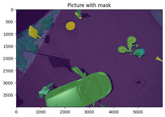
Display one image associated with the mask to clearly understand how the objects are segmented into the image. The image size is (4000, 6000,3) which is very high resolution.

# Display an image with mask
img = Image.open(image_path + df['id'][101] + '.jpg')
mask = Image.open(mask_path + df['id'][101] + '.png')
print('Image size', np.asarray(img).shape)
print('mask size', np.asarray(mask).shape)
plt.imshow(img)
plt.imshow(mask, alpha= 0.6)
plt.title("Picture with mask")
plt.show()
Image size (4000, 6000, 3) 
mask size (4000, 6000)

Now split the data into train, test and validation dataset. You can see the number of samples are using in training, validation and testing in the result. 

# split the data
X_trainval, X_test = train_test_split(df['id'].values, test_size=0.1, random_state=42)
X_train, X_val = train_test_split(X_trainval, test_size= 0.15, random_state=42)
print('Train Size : ', len(X_train))
print('Val Size : ', len(X_val))
print('Test Size : ', len(X_test))
Train Size : 306 
Val Size : 54 
Test Size : 40

“DroneDataset” is a custom dataset class that is used to load images and their corresponding segmentation masks. “__getitem__” is responsible for loading and preprocessing individual samples from the dataset. “Tiles” is used to extract image patches and corresponding mask patches from the loaded images and masks. It divides the images and mask into smaller patches of specified dimensions(512*768) and reshape them that look like (n, 3, 512, 768) where n is the number of patches.

# Dataset
class DroneDataset(Dataset):
    def __init__(self, img_path, mask_path, X, mean, std, transform = None, patch = False):
        self.img_path = img_path		# path of the image dataset
        self.mask_path = mask_path		# path of mask dataset
        self.X = X  				# list of image file names
        self.mean = mean				# used for image normalisation
        self.std = std				# same as mean
	  #optional for image and mask augmentation
        self.transform = transform	        
 	  self.patches = patch			# does image patches yes or not
    # define the len of the data
    def __len__(self):
        return len(self.X)
    def __getitem__(self, idx):
        img = cv2.imread(self.img_path + self.X[idx] + '.jpg')
        img = cv2.cvtColor(img, cv2.COLOR_BGR2RGB)
        mask = cv2.imread(self.mask_path + self.X[idx] + '.png', cv2.IMREAD_GRAYSCALE)
        if self.transform is not None:
            aug = self.transform(image = img, mask= mask)
            img = Image.fromarray(aug['image'])
            mask = aug['mask']
        if self.transform is None:
            img = Image.fromarray(img)
        t = T.Compose([T.ToTensor(), T.Normalize(self.mean, self.std)])
        img = t(img)
        mask = torch.from_numpy(mask).long()
        if self.patches:
            img, mask = self.tiles(img, mask)
        return img, mask
    def tiles(self, img, mask):
        img_patches = img.unfold(1,512,512).unfold(2,768,768)
        img_patches = img_patches.contiguous().view(3,-1,512,768)
        img_patches = img_patches.permute(1,0,2,3)
        mask_patches = mask.unfold(0,512, 512).unfold(1,768,768)
        mask_patches = mask_patches.contiguous().view(-1,512,768)
        return img_patches, mask_patches

This block is used for define data augmentation, creating dataset instances and data loader. ‘T_train’ and ‘t_val’ are used to define data augmentation techniques using the Albumentation library. It is used to increase the diversity of the training data and improve the generalisation of deep learning models. ‘Mean’ and ‘std’ are used in image normalisation. We have been using a number of data augmentation techniques such as resize images with nearest neighbour method, horizontal flipping, vertical flipping, grid distortion with 20% probability, random brightness and adjust contrast, adding gaussian noise. ‘Train Set’ and ‘valset’ define the training dataset and validation dataset. Then using the data loader function, we create the data batch for an efficient process. It is essential for iterating data through training and validation datasets, that allow to train the model in mini batches and accelerate training and help control memory usage.

# Apply transformation
mean = [0.485, 0.456, 0.406]
std = [0.229, 0.224, 0.225]
t_train = A.Compose([A.Resize(704,1056, interpolation=cv2.INTER_NEAREST),
                     A.HorizontalFlip(),
                     A.VerticalFlip(),
                     A.GridDistortion(p=0.2),
                     A.RandomBrightnessContrast((0,0.5),(0,0.5)),
                     A.GaussNoise()])
t_val = A.Compose([A.Resize(704, 1056, interpolation=cv2.INTER_NEAREST),
                    A.HorizontalFlip(),
                    A.GridDistortion(p=0.2)])
# datasets
train_set = DroneDataset(image_path, mask_path,X_train,mean,std,t_train, patch = False)
val_set = DroneDataset(image_path, mask_path, X_val, mean, std, t_val, patch = False)
print(len(val_set))
# dataloader
batch_size = 3
train_loader = DataLoader(train_set, batch_size=batch_size, shuffle=True)
val_loader = DataLoader(val_set, batch_size = batch_size, shuffle= True)
54
Our dataset is ready for training. Now take a batch of images and labels and see the size of the dataset.
# Display image and label.
train_features, train_labels = next(iter(train_loader))
print(f"Feature batch shape: {train_features.size()}")
print(f"Labels batch shape: {train_labels.size()}")
Feature batch shape: torch.Size([3, 3, 704, 1056]) 
Labels batch shape: torch.Size([3, 704, 1056])

Define Unit Model

We define the UNet model from segmentation_models_pytorch library and choose mobilenet_v2 as a backbone architecture of UNet. Pretrained imagenet weights have been specified. Activation is None that will be applied to the model’s final output. ‘encoder _depth’ defines the depth of the encoder that captures more abstract features. ‘decoder _channels’ defines the number of channels in the decoder part. 

In a summary, we define a UNet based segmentation model with MobileNetV2 as the backbone, using pre-trained weights from ImageNet and the model is configured for segmentation tasks with 23 classes.

# model
model = smp.Unet('mobilenet_v2', encoder_weights= 'imagenet',classes= 23, activation = None,
                    encoder_depth = 5,
                    decoder_channels = [256,128,64, 32, 16])
print(model)

This function calculates the pixel accuracy between the model’s segmentation output and the ground truth mask. 

# training
def pixel_accuracy(output, mask):
    with torch.no_grad():
        output = torch.argmax(F.softmax(output, dim=1), dim=1)
        correct = torch.eq(output, mask).int()
        accuracy = float(correct.sum()) / float(correct.numel())
    return accuracy

This function is used to calculate the mean IoU score between predicted segmentation masks and ground truth masks for multi class segmentation tasks. 

# mean IoU
def mIoU(pred_mask, mask, smooth=1e-10, n_classes=23):
    with torch.no_grad():
        pred_mask = F.softmax(pred_mask, dim=1)
        pred_mask = torch.argmax(pred_mask, dim =1)
        pred_mask = pred_mask.contiguous().view(-1)
        mask = mask.contiguous().view(-1)
        iou_per_class = []
        for clas in range(0, n_classes):
            true_class = pred_mask ==clas
            true_label = mask == clas
            if true_label.long().sum().item() == 0:
                iou_per_class.append(np.nan)
            else:
                intersect = torch.logical_and(true_class, true_label).sum().float().item()
                union = torch.logical_or(true_class, true_label).sum().float().item()
                iou = (intersect + smooth) / (union + smooth)
                iou_per_class.append(iou)
        return np.nanmean(iou_per_class)

This simple function is used to retrieve the current learning rate from an optimizer.

def get_lr(optimizer):
    for param_group in optimizer.param_groups:
        return param_group['lr']

Train the model

The fit function is used to train a segmentation model over multiple epochs using the specified training and validation data and monitor the training process and save the model under certain conditions.

def fit(epochs, model, train_loader, val_loader, criterion, optimizer, scheduler, patch=False):
    torch.cuda.empty_cache()
    train_losses = []
    test_losses = []
    val_iou = []; val_acc = []
    train_iou = []; train_acc = []
    lrs = []
    min_loss = np.inf
    decrease = 1 ; not_improve=0
    model.to(device)
    fit_time = time.time()
    for e in range(epochs):
        since = time.time()
        running_loss = 0
        iou_score = 0
        accuracy = 0
        #training loop
        model.train()
        for i, data in enumerate(tqdm(train_loader)):
            #training phase
            image_tiles, mask_tiles = data
            if patch:
                bs, n_tiles, c, h, w = image_tiles.size()
                image_tiles = image_tiles.view(-1,c, h, w)
                mask_tiles = mask_tiles.view(-1, h, w)
           
            image = image_tiles.to(device); mask = mask_tiles.to(device);
            #forward
            output = model(image)
            loss = criterion(output, mask)
            #evaluation metrics
            iou_score += mIoU(output, mask)
            accuracy += pixel_accuracy(output, mask)
            #backward
            loss.backward()
            optimizer.step() #update weight          
            optimizer.zero_grad() #reset gradient
           
            #step the learning rate
            lrs.append(get_lr(optimizer))
            scheduler.step()
           
            running_loss += loss.item()
           
        Else:
		# similar to training phase but without gradient calculations
		# metrics and losses are computed for validation data.
            model.eval()
            test_loss = 0
            test_accuracy = 0
            val_iou_score = 0
            #validation loop
            with torch.no_grad():
                for i, data in enumerate(tqdm(val_loader)):
                    #reshape to 9 patches from single image, delete batch size
                    image_tiles, mask_tiles = data
                    if patch:
                        bs, n_tiles, c, h, w = image_tiles.size()
                        image_tiles = image_tiles.view(-1,c, h, w)
                        mask_tiles = mask_tiles.view(-1, h, w)
                   
                    image = image_tiles.to(device); mask = mask_tiles.to(device);
                    output = model(image)
                    #evaluation metrics
                    val_iou_score +=  mIoU(output, mask)
                    test_accuracy += pixel_accuracy(output, mask)
                    #loss
                    loss = criterion(output, mask)                                  
                    test_loss += loss.item()
           
            #calculatio mean for each batch
            train_losses.append(running_loss/len(train_loader))
            test_losses.append(test_loss/len(val_loader))

            if min_loss > (test_loss/len(val_loader)):
                print('Loss Decreasing.. {:.3f} >> {:.3f} '.format(min_loss, (test_loss/len(val_loader))))
                min_loss = (test_loss/len(val_loader))
                decrease += 1
                if decrease % 5 == 0:
                    print('saving model...')
                    torch.save(model, 'Unet-Mobilenet_v2_mIoU-{:.3f}.pt'.format(val_iou_score/len(val_loader)))
                   
            if (test_loss/len(val_loader)) > min_loss:
                not_improve += 1
                min_loss = (test_loss/len(val_loader))
                print(f'Loss Not Decrease for {not_improve} time')
                if not_improve == 7:
                    print('Loss not decrease for 7 times, Stop Training')
                    break
           
            #iou
            val_iou.append(val_iou_score/len(val_loader))
            train_iou.append(iou_score/len(train_loader))
            train_acc.append(accuracy/len(train_loader))
            val_acc.append(test_accuracy/ len(val_loader))
            print("Epoch:{}/{}..".format(e+1, epochs),
                  "Train Loss: {:.3f}..".format(running_loss/len(train_loader)),
                  "Val Loss: {:.3f}..".format(test_loss/len(val_loader)),
                  "Train mIoU:{:.3f}..".format(iou_score/len(train_loader)),
                  "Val mIoU: {:.3f}..".format(val_iou_score/len(val_loader)),
                  "Train Acc:{:.3f}..".format(accuracy/len(train_loader)),
                  "Val Acc:{:.3f}..".format(test_accuracy/len(val_loader)),
                  "Time: {:.2f}m".format((time.time()-since)/60))
       
    history = {'train_loss' : train_losses, 'val_loss': test_losses,
               'train_miou' :train_iou, 'val_miou':val_iou,
               'train_acc' :train_acc, 'val_acc':val_acc,
               'lrs': lrs}
    print('Total time: {:.2f} m' .format((time.time()- fit_time)/60))
    return history

Loss Decreasing.. inf >> 1.408 
Epoch:1/15.. Train Loss: 1.888.. Val Loss: 1.408.. Train mIoU:0.099.. Val mIoU: 0.125.. Train Acc:0.547.. Val Acc:0.668.. Time: 2.05m
Loss Decreasing.. 1.408 >> 1.164 
Epoch:2/15.. Train Loss: 1.547.. Val Loss: 1.164.. Train mIoU:0.120.. Val mIoU: 0.142.. Train Acc:0.593.. Val Acc:0.683.. Time: 2.04m
—--------------------------------------------------------------------------------
—--------------------------------------------------------------------------------
Loss Decreasing.. 0.594 >> 0.571 
Epoch:13/15.. Train Loss: 0.702.. Val Loss: 0.571.. Train mIoU:0.285.. Val mIoU: 0.306.. Train Acc:0.787.. Val Acc:0.830.. Time: 2.10m
Loss Decreasing.. 0.571 >> 0.567 
Epoch:14/15.. Train Loss: 0.699.. Val Loss: 0.567.. Train mIoU:0.289.. Val mIoU: 0.311.. Train Acc:0.790.. Val Acc:0.833.. Time: 2.05m
Loss Decreasing.. 0.567 >> 0.552 
saving model...
Epoch:15/15.. Train Loss: 0.690.. Val Loss: 0.552.. Train mIoU:0.291.. Val mIoU: 0.311.. Train Acc:0.792.. Val Acc:0.837.. Time: 2.05m
Total time: 30.65 m

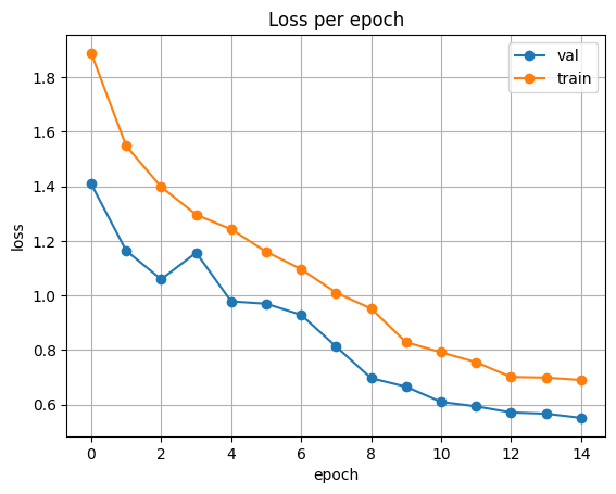
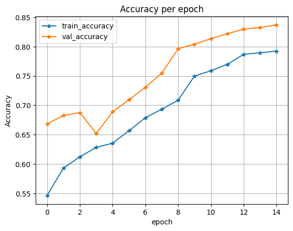
The following three plotting functions are used to visualise training and validation loss, score and accuracy after training a segmentation model. ‘Plot_loss’ function takes the history of the trained model and visualises the loss of training and validation over time. ‘Plot score’ gives visualisation of the score of Mean Iou for both training and validation data. ‘Plot_acc’ visualises the accuracy per epoch of both training and validation. 

#torch.save(model, 'Unet-Mobilenet.pt')
def plot_loss(history):
    plt.plot(history['val_loss'], label='val', marker='o')
    plt.plot( history['train_loss'], label='train', marker='o')
    plt.title('Loss per epoch'); plt.ylabel('loss');
    plt.xlabel('epoch')
    plt.legend(), plt.grid()
    plt.show()
   
def plot_score(history):
    plt.plot(history['train_miou'], label='train_mIoU', marker='*')
    plt.plot(history['val_miou'], label='val_mIoU',  marker='*')
    plt.title('Score per epoch'); plt.ylabel('mean IoU')
    plt.xlabel('epoch')
    plt.legend(), plt.grid()
    plt.show()
   
def plot_acc(history):
    plt.plot(history['train_acc'], label='train_accuracy', marker='*')
    plt.plot(history['val_acc'], label='val_accuracy',  marker='*')
    plt.title('Accuracy per epoch'); plt.ylabel('Accuracy')
    plt.xlabel('epoch')
    plt.legend(), plt.grid()
    plt.show()

Now see the loss function, MIoU and accuracy metrics for more understanding about the training condition of the model.

plot_loss(history)
plot_score(history)
plot_acc(history)

Evaluation Part

This dataset is designed for use in testing or inference with a segmentation model where ‘__getitem__’ method is responsible for loading and processing a single given index ’idx’. 

class DroneTestDataset(Dataset):
   
    def __init__(self, img_path, mask_path, X, transform=None):
        self.img_path = img_path
        self.mask_path = mask_path
        self.X = X
        self.transform = transform
     
    def __len__(self):
        return len(self.X)
   
    def __getitem__(self, idx):
        img = cv2.imread(self.img_path + self.X[idx] + '.jpg')
        img = cv2.cvtColor(img, cv2.COLOR_BGR2RGB)
        mask = cv2.imread(self.mask_path + self.X[idx] + '.png', cv2.IMREAD_GRAYSCALE)
       
        if self.transform is not None:
            aug = self.transform(image=img, mask=mask)
            img = Image.fromarray(aug['image'])
            mask = aug['mask']
       
        if self.transform is None:
            img = Image.fromarray(img)
       
        mask = torch.from_numpy(mask).long()
       
        return img, mask

Create a test dataset (‘test_set’) by initialising an instance of the DroneTestDataset class with the provided parameters and ‘t_test’ is used for resizing the images.

t_test = A.Resize(768, 1152, interpolation=cv2.INTER_NEAREST)
test_set = DroneTestDataset(image_path, mask_path, X_test, transform=t_test)

This function is designed to take a single test image,perform inference using a segmentation model and compute IoU score to assess the model’s performance on that image. 

def predict_image_mask_miou(model, image, mask, mean=[0.485, 0.456, 0.406], std=[0.229, 0.224, 0.225]):
    model.eval()
    t = T.Compose([T.ToTensor(), T.Normalize(mean, std)])
    image = t(image)
    model.to(device); image=image.to(device)
    mask = mask.to(device)
    with torch.no_grad():
       
        image = image.unsqueeze(0)
        mask = mask.unsqueeze(0)
       
        output = model(image)
        score = mIoU(output, mask)
        masked = torch.argmax(output, dim=1)
        masked = masked.cpu().squeeze(0)
    return masked, score

This function is used to predict a single test image and compute the pixel accuracy to assess the model’s performance on that image.It returns predicted segmentation mask and the pixel accuracy.

def predict_image_mask_pixel(model, image, mask, mean=[0.485, 0.456, 0.406], std=[0.229, 0.224, 0.225]):
    model.eval()
    t = T.Compose([T.ToTensor(), T.Normalize(mean, std)])
    image = t(image)
    model.to(device); image=image.to(device)
    mask = mask.to(device)
    with torch.no_grad():
       
        image = image.unsqueeze(0)
        mask = mask.unsqueeze(0)
       
        output = model(image)
        acc = pixel_accuracy(output, mask)
        masked = torch.argmax(output, dim=1)
        masked = masked.cpu().squeeze(0)
    return masked, acc

image, mask = test_set[3]

pred_mask, score = predict_image_mask_miou(model, image, mask)

The ‘miou_score’ function is used to calculate the mean Intersection over Union(mIoU) scores to evaluate the segmentation model’s performance in the entire test dataset.

def miou_score(model, test_set):
    score_iou = []
    for i in tqdm(range(len(test_set))):
        img, mask = test_set[i]
        pred_mask, score = predict_image_mask_miou(model, img, mask)
        score_iou.append(score)
    return score_iou
mob_miou = miou_score(model, test_set)

The pixel_acc function allows you to evaluate the segmentation model’s performance on the entire test dataset by calculating the pixel accuracy for each image. 

def pixel_acc(model, test_set):
    accuracy = []
    for i in tqdm(range(len(test_set))):
        img, mask = test_set[i]
        pred_mask, acc = predict_image_mask_pixel(model, img, mask)
        accuracy.append(acc)
    return accuracy
mob_acc = pixel_acc(model, test_set)

Now Visualise the main image, its corresponding mask and the predicted mask through the segmentation model.

fig, (ax1, ax2, ax3) = plt.subplots(1,3, figsize=(20,10))
ax1.imshow(image)
ax1.set_title('Picture');
ax2.imshow(mask)
ax2.set_title('Ground truth')
ax2.set_axis_off()
ax3.imshow(pred_mask)
ax3.set_title('UNet-MobileNet | mIoU {:.3f}'.format(score))
ax3.set_axis_off()

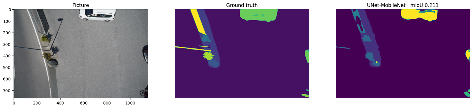
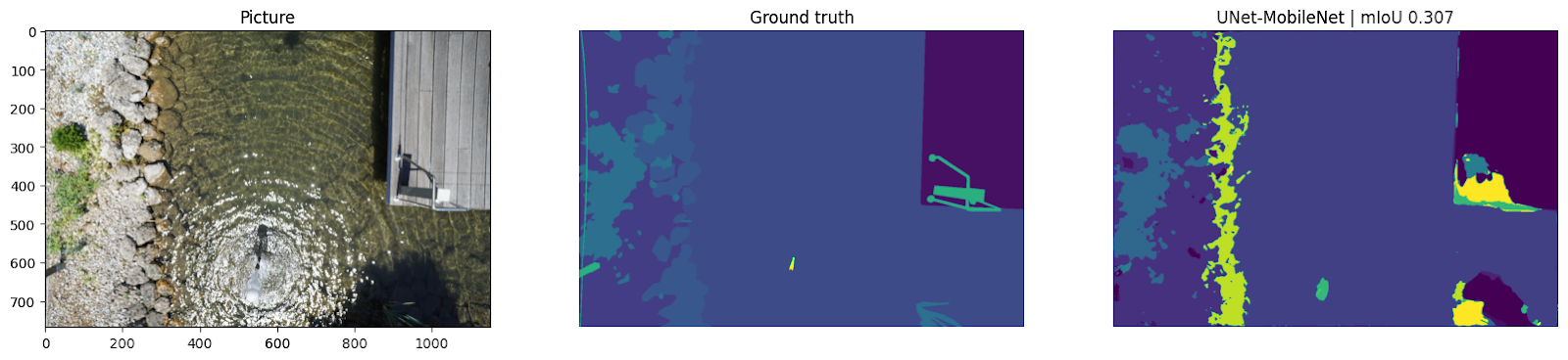
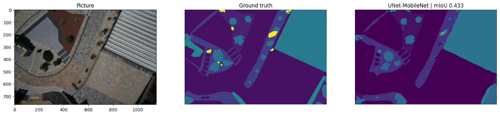
print('Test Set mIoU', np.mean(mob_miou))
Test Set mIoU 0.3417332485424927
print('Test Set Pixel Accuracy', np.mean(mob_acc))
Test Set Pixel Accuracy 0.8475476582845053

Challenges and Strategies

Image segmentation is a popular technique in computer vision but it still presents various challenges. Some of the challenges and strategies to overcome the challenge is given below. 

• Ambiguity and Variability: Image can be ambiguous and variations in lighting, then use advanced deep learning based methods to capture complex patterns and context.
• Over-segmentation and under- segmentation: Many algorithms struggle with finding the right balance between over segmentation and under segmentation. To overcome this issue, consider post processing techniques to merge or split regions as needed and explore region merging and region growing algorithms.
• Occlusions: It occurs in image when objects partially or fully block by others. To overcome, investigate methods for handling occlusions such as use 3D data or adopting instance segmentation techniques and others.
• Real time processing: For real time image segmentation, algorithms need to be computationally efficient. So, use lightweight network architecture and increase hardware acceleration.
• Handling high or large resolution images: It needs high computational resources and memory. So you can implement image tiling or patch based approaches (SAHI) to process large images in smaller sections. 
• Fine Grained Segmentation: Distinguishing fine details or fine grained textures can be challenging. So, employ models capable of capturing fine grained features, and consider post processing techniques like boundary refinement or pixel wise conditional random fields and others. 
• Domain adaptation: Models trained on one domain may not generalise will to new or different domains. So, explore domain adaptation techniques to fine tune models for specific domains or datasets.
• Evaluation Metrics: Selecting appropriate evaluation metrics can be challenging. So, use evaluation metrics like intersection over union(IoU), pixel accuracy, F1 score for assessing the quality of segmentation results and choose metrics that align with the specific objectives of your application.

There may be other challenges over time. Try to fix those issues and explore others.

Deploy segmentation models

We have already created the segmentation model. Now it is prepared for real world scenarios. We can integrate our model into web applications, mobile apps or others. There are some ways that can be used for development of the model.

• Export the trained model in a format that can be loaded in deployment environments such as Tensorflow saved model, PyTorch JIT script, ONNX and others.
• Choose the deployment environment. That may be a cloud based platform, an edge device, server or others.
• For cloud, AWS, Google Cloud Platform(GCP), Microsoft Azure or others can be taken. Containerize the model using Docker and deploy the model as a web service like AWS Lambda, AWS SageMaker, Google Cloud Functions, Azure Functions or others. Then expose an API that can be accessed from a web application or mobile app.
• For edge devices like mobile phones, IoT devices or embedded systems, we can use Tensorflow lite(Android) or Core ML(ios) to run locally on the device.
• For model serving, we can use Tensorflow Serving, TorchServe or ONXX runtime to serve the model through RESTful APIs. 
• Set up monitoring and logging for the deployed model to track usage, performance and errors.
• Thoroughly test the deployed model to ensure it performs as expected in the production environment.
• Regularly update the model with new data and retrain it as needed to improve performance.

One thing is to remember that deployment is an ongoing process. So, regularly monitor and update the deployment to address changes in data distribution, user requirements and potential security threats.

We have explored the fundamental concept, methods, real world applications, traditional image segmentation and deep learning based image segmentation techniques. We also discussed challenges in image segmentation and how to overcome it. Then we implement a real world semantic segmentation problem with the UNet model. Then some discussion of deployment has been done. Overall, this article gives you the concept of image segmentation. 

This is not the whole thing about image segmentation, the guide encourages further exploration into advanced segmentation topics like panoptic segmentation and advanced algorithms like Deeplabv3, yolo7 or others. Researchers and developers are encouraged to delve into video segmentation, which involves segmenting objects and regions in video sequences. There are many opportunities to develop more efficient algorithms, improve model accuracy, and address the challenges by staying up to date with the latest advancements and research. Hope, You gain some knowledge and wanna to go further. Happy Learning!!!!