Hands-on Image Classification in Computer Vision | Computer Vision

Image classification is the fundamental task in computer vision. It is a crucial duty in machine learning and computer vision that involves assigning predefined labels to images based on visual content. In this tutorial, we will describe image classification using real-world applications and a classification architecture.

Real-World Examples:

Image classification using Modern World in various fields, from healthcare to space. Here are some examples:

Autonomous Vehicles: Self-driving cars are a hot topic in the current world. Tesla, Google, Apple, and other tech giants are racing in this auto-driving competition.  Image classification is used as the core label for autopilot. For object classification and detection of multiple objects in a single short, It uses image classification to recognize pedestrians, road signs, and other vehicles to make real-time decisions.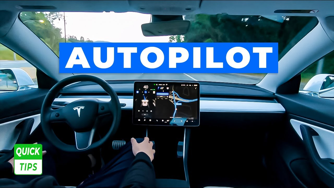

Understanding Image Classification: Image classification involves assigning a label to an image from a set of predefined categories. In machine learning,  An essential function is image classification, which involves selecting a specific label for a picture from a specified set of categories. This fundamental procedure is the cornerstone for creating increasingly complex and sophisticated applications spanning numerous disciplines and industries. It serves as a fundamental task, paving the way for more complex applications.

Applications: Image classification is used in various sectors.  Here are some of them.

Sentiment Analysis: Numerous applications, such as market research, customer feedback analysis, and mental health monitoring, are well suited for this skill. The correct classification of facial expressions into emotional states, including happiness, sadness, rage, and more, through image classification plays a vital role in sentiment analysis.

Wildlife Conservation: Image categorization provides a powerful technique for recognizing distinct species in ecology and wildlife protection. Researchers and conservationists may quickly collect data for biodiversity studies, habitat protection, and population monitoring by automating the process of species identification through pictures.

Quality Control: It makes quality control procedures more accessible, and picture classification benefits the industrial sector. Manufacturers may increase their production effectiveness, reduce waste, and uphold better quality standards by quickly and accurately identifying product flaws on assembly lines.

Choosing the Right Model: Convolutional Neural Networks (CNNs) are the backbone of image classification. LeNet, AlexNet, VGGNet, ResNet, and Inception are popular architectures, each with unique design principles. The model choice should align with the dataset size and complexity.

Popular CNN Architectures:

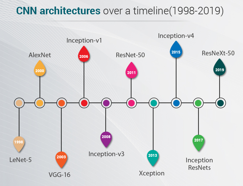
In 1998, LeNet architecture was developed by Yann LeCun et al. with a 5-layer architecture. LeNet was crucial in explaining the effectiveness of CNNs in picture classification tasks, motivating the creation of more complex structures, and laying the groundwork for current deep learning-based computer vision applications. In 2000, AlexNet was developed; it had an 8-layer architecture with 60 million parameters. After that, In 2014 Visual Geometry Group at the University of Oxford created the popular VGG-16  model, VGG-16 has 13 convolutional and 3 fully connected layers and has 138 million parameters. Google has also developed Inception v1, also known as GoogleNet. In 2016, Release DenseNet, its layers are highly connected dense blocks. Day by day, several architectures are developed by AlexNet and are continuously developed. 

Model Selection Considerations: In this tutorial, we will implement the coding part using Rsenet50. Resnet 50 is good work for large datasets. The competitive performance of ResNet-50 in image classification tasks is well recognized. It offers a solid baseline for  CIFAR-10 classification work and has received top rankings in several benchmark tests.

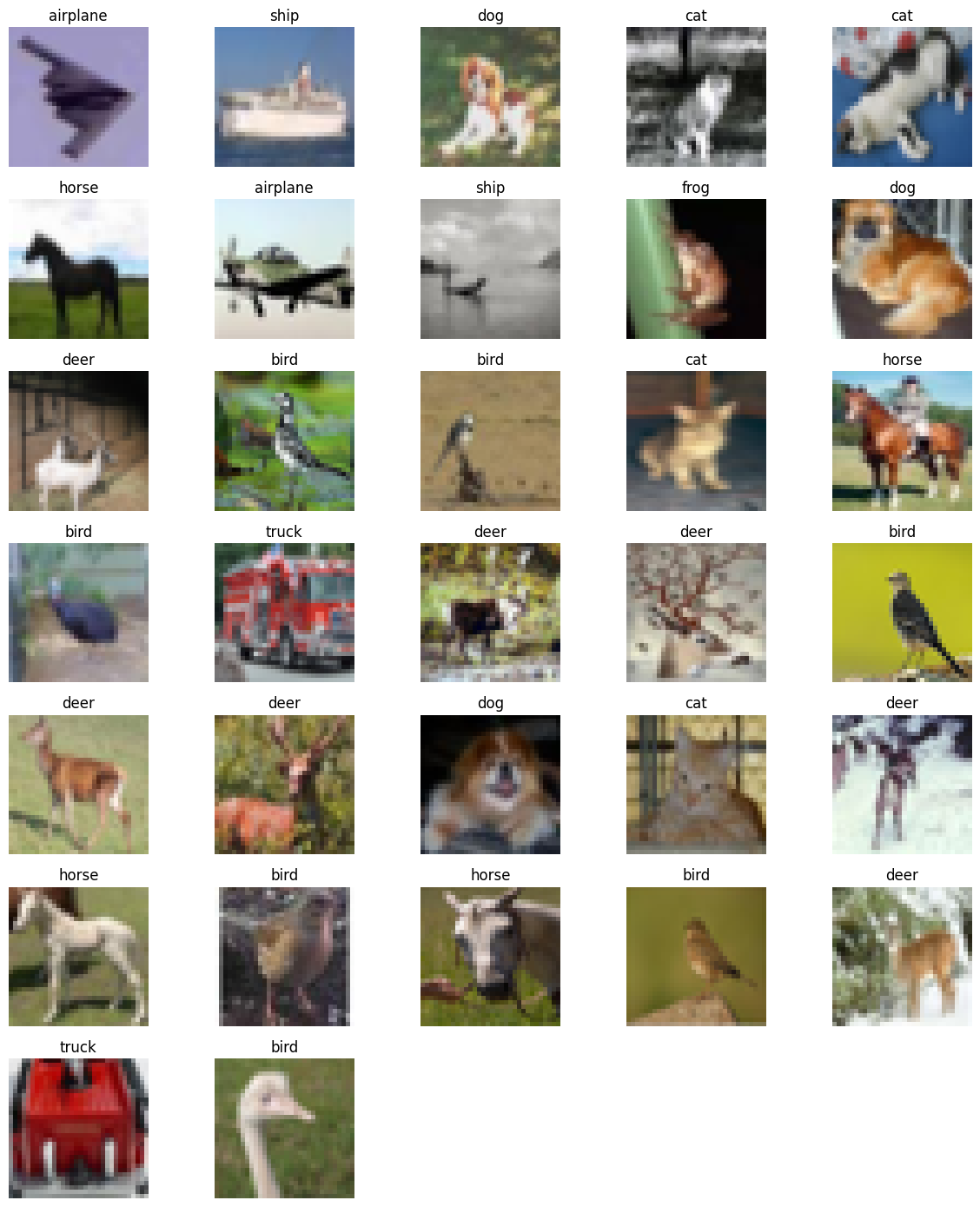
Dataset Size: In our implementation part, we will use the CIFAR-10 dataset. It is an amazing dataset for image classification. It has ten classes of images. The dataset contains 60,000 32x32 color images in 10 different classes, with 6,000 images per class. The size of the dataset is 170 MB.

Complexity: Rsenet50 has a 50-layer architecture, which means it can handle more complex features from input data.

Data Acquisition and Preparation: 

We use popular libraries like PyTorch to load the CIFAR-10 dataset. You will get the full project code on Google Colab. Below are examples using this library:

# Import necessary libraries
import torch  
# Import the main PyTorch library
import torch.nn as nn 
# Import PyTorch's neural network module
import torch.optim as optim  
# Import PyTorch's optimization module
import torchvision  
# Import the torchvision library for computer vision tasks
import torchvision.transforms as transforms  
# Import image transformation functions
import torchvision.models as models  
# Import pre-defined deep learning models

Data Pipeline and Preprocessing: 

Loading Data: In our implementation part, we used the CIFAR-10 dataset. CIFAR-10 is often used as a benchmark dataset for testing and developing image classification models.

# Define data transformations and load the CIFAR-10 dataset
transform = transforms.Compose([
    # Data augmentation: random horizontal flip and random crop with padding
    transforms.RandomHorizontalFlip(),
    transforms.RandomCrop(32, padding=4),
    transforms.ToTensor(),  # Convert images to PyTorch tensors
    transforms.Normalize(mean=[0.485, 0.456, 0.406], std=[0.229, 0.224, 0.225])  # Normalize pixel values
])
# Load CIFAR-10 training dataset
# The 'transform' argument specifies the data transformations to be applied to the images, as defined in the previous code block.
trainset = torchvision.datasets.CIFAR10(root='./data', train=True, download=True, transform=transform)
# 'batch_size=128' specifies that each batch will contain 128 images. 'shuffle=True' indicates that the order of the data
# within each batch will be shuffled during training, which helps in randomizing the order of training examples.
trainloader = torch.utils.data.DataLoader(trainset, batch_size=128, shuffle=True)
# Load CIFAR-10 test dataset
# This line loads the CIFAR-10 test dataset. Similar to the training dataset, it specifies the root directory, sets 'train=False'
# to indicate that we want the test split of the dataset, and uses the same 'transform' as the training dataset.
testset = torchvision.datasets.CIFAR10(root='./data', train=False, download=True, transform=transform)
# This line creates a data loader for the test dataset. It follows the same principles as the training data loader but is used for
# evaluating the model's performance on unseen data, which is the purpose of the test dataset.
testloader = torch.utils.data.DataLoader(testset, batch_size=128, shuffle=False)

Building  Classification Model:  We will build a classification model using ResNet-50 CNN-based architecture. Here is the  coding part:

# Define the ResNet-50 model
resnet50 = models.resnet50(pretrained=False)
resnet50.fc = nn.Linear(resnet50.fc.in_features, 10)  # Change the output layer to have 10 classes
# Define loss function and optimizer
criterion = nn.CrossEntropyLoss()
optimizer = optim.SGD(resnet50.parameters(), lr=0.01, momentum=0.9, weight_decay=1e-4)
# Move the model and data to GPU if available
device = torch.device("cuda" if torch.cuda.is_available() else "cpu")
resnet50.to(device)
# Training loop
num_epochs = 80
for epoch in range(num_epochs):
    running_loss = 0.0
    for i, data in enumerate(trainloader, 0):
        inputs, labels = data
        inputs, labels = inputs.to(device), labels.to(device)
        optimizer.zero_grad()
        outputs = resnet50(inputs)
        loss = criterion(outputs, labels)
        loss.backward()
        optimizer.step()
        running_loss += loss.item()
    print(f"Epoch {epoch+1}/{num_epochs}, Loss: {running_loss / (i+1):.4f}")
print("Finished Training")

Model Training: Here is the model  training part of this implementation.

# Number of training epochs, typically set to a predefined value.
num_epochs = 80
# Loop over the specified number of training epochs.
for epoch in range(num_epochs):
    
    # Initialize a running loss variable to keep track of the cumulative loss during the epoch.
    running_loss = 0.0
    
    # Iterate over batches of data from the training data loader.
    for i, data in enumerate(trainloader, 0):
        
        # Unpack the batch into inputs (images) and labels.
        inputs, labels = data
        
        # Move the batch to the device (e.g., GPU) if available, enabling faster computation.
        inputs, labels = inputs.to(device), labels.to(device)
        
        # Zero the gradients of the model's parameters to avoid accumulating gradients from previous iterations.
        optimizer.zero_grad()
        
        # Forward pass: Compute model predictions (outputs) for the input batch.
        outputs = resnet50(inputs)
        
        # Compute the loss between the model's predictions and the ground truth labels.
        loss = criterion(outputs, labels)
        
        # Backpropagate the gradients and update the model's parameters.
        loss.backward()
        optimizer.step()
        
        # Accumulate the current batch's loss to the running loss.
        running_loss += loss.item()
    
    # Print the average loss for the current epoch.
    print(f"Epoch {epoch+1}/{num_epochs}, Loss: {running_loss / (i+1):.4f}")
# Training loop completed.
print("Finished Training")
# Initialize variables to keep track of correct predictions and the total number of test samples.
correct = 0
total = 0
# Disable gradient computation during testing to save memory and computation.
with torch.no_grad():
    
    # Iterate over batches of data from the test data loader.
    for data in testloader:
        
        # Unpack the batch into inputs (images) and labels.
        inputs, labels = data
        
        # Move the batch to the device (e.g., GPU) if available, enabling faster computation.
        inputs, labels = inputs.to(device), labels.to(device)
        
        # Perform a forward pass to compute model predictions (outputs) for the input batch.
        outputs = resnet50(inputs)
        
        # Find the class with the highest predicted probability for each sample in the batch.
        _, predicted = torch.max(outputs.data, 1)
        
        # Update the total count of test samples.
        total += labels.size(0)
        
        # Count the number of correct predictions by comparing predicted labels to ground truth labels.
        correct += (predicted == labels).sum().item()
# Calculate the accuracy by dividing the number of correct predictions by the total number of test samples.
accuracy = (100 * correct / total)
# Print the accuracy on the test set.
print(f"Accuracy on the test set: {accuracy:.2f}%")

In this tutorial, we try to cover the basic image classification, the application of image classification, and implementation using ResNet 50. For more details and depth learning, you can follow this course.