- Introduction to Computer Vision
- Image Preprocessing for Computer Vision
- Mathematical Analysis for Computer Vision
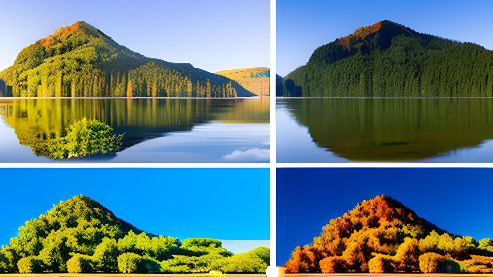
- A Complete Guide of Data Augmentation in Computer Vision
- Hands-on Image Classification in Computer Vision
- Face Recognition in Computer Vision with Implementation
- A Complete Guide to Object Detection with Implementation in Computer Vision
- A Comprehensive Guide to Image Segmentation in Computer Vision
- Pose Estimation in Computer Vision: Concepts & Implementation
- Optical Character Recognition (OCR) in Computer Vision: From Pixels to Text
- Image Generation with DCGANs in Computer Vision
- A Complete Guide to Image Restoration in Computer Vision
- 3D image generation in Computer Vision with implementation
Image Preprocessing for Computer Vision | Computer Vision
Image data Preprocessing is an essential method that underpins the success of different computer vision tasks and applications. In this tutorial, we will discuss the importance of image processing, some preprocessing tools, and some preprocessing techniques. So let's deep dive into it.
Importance of Image Preprocessing
Image preprocessing plays a pivotal role in computer vision tasks due to the following reasons:
Enhanced Data Quality: Raw images can include noise, antiques, or inconsistencies that slow the model version. Preprocessing manages these issues to provide cleaner and more reliable data.
Improved Model Performance: Clean and standardized data allows models to learn meaningful patterns more effectively, resulting in better predictive performance and generalization.
Reduced Model Complexity: Proper preprocessing simplifies data by removing redundancies or irrelevant information, leading to more efficient models requiring fewer computational resources.
Tools and Platforms:
OpenCV: OpenCV is open-source software for computer vision and image processing activities. It has a Python interface and is developed in C++, making it simple to include in Python applications. With the help of OpenCV, programmers can manipulate images and videos and perform tasks like object detection, facial recognition, and image editing. It is widely utilized in various industries, including robotics, research, and image processing, because of its adaptable features and built-in algorithms. You can learn more about openCV from there official documentation.
Keras: Python-based, user-friendly Keras is an open-source neural network API image processing technique. It was initially independently created and is now a part of the TensorFlow ecosystem. Providing an explicit interface and a modular design streamlines deep learning models' creation, training, and deployment. Keras enables custom layers, loss functions, and metrics, highlighting flexibility. While it initially supported various backends, TensorFlow is now deeply integrated. Keras is preferred for quick experimentation since it gives users access to pre-trained models and makes it possible to design unique structures.
Image Data Basics:
Image data is represented with a height and width based on the number of pixels. such as 600 X 400 images, the total number of pixels is 240000. There are three types of images, according to pixels.Grayscale: An integer with a value of 0 to 255, or totally black or completely white, is called a grayscale.
RGB: The three integers, which range from 0 to 255 and represent the intensity of red, green, and blue, make up a pixel.
RGBA: It is a modification of RGB with an additional alpha field, which stands for the image's opacity.
Challenges: Complexity, Accuracy
Due to differences in lighting, angles, and backdrops, image data might be complex. Image preprocessing seeks to standardize these differences for consistent input. Furthermore, image preprocessing ensures the integrity of the data; avoiding bias or misinterpretation depends on accurate preparation.
Image Preprocessing Goals
Clean Data Formatting: It is an essential way to prepare data consistently. These techniques include scaling down photographs to a standard size and pruning out irrelevant pieces to guarantee uniformity and eliminate distractions.
Improved Model Performance: Enhancing contrast, reducing noise, and emphasizing appropriate features through preprocessing contribute to better model performance. Models trained on preprocessed data can learn more effectively.
Simplified Model Complexity: Removing noise and irrelevant details simplifies the data, allowing models to focus on important information. This shows faster training times and more efficient inference.
Loading Data:
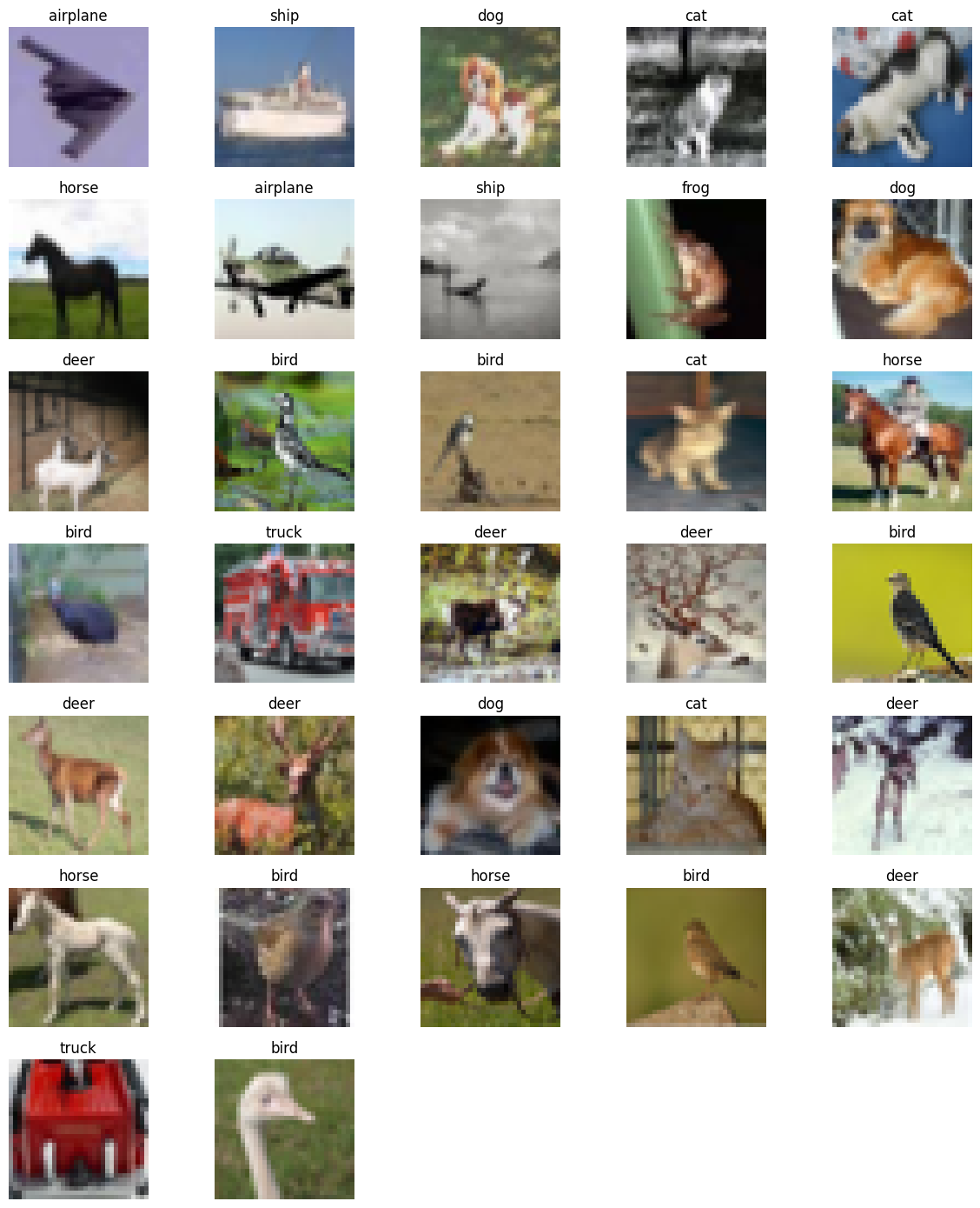
We will use the CIFAR-10 dataset. CIFAR-10 is often used as a benchmark dataset for testing and developing image classification models. The dataset contains 60,000 32x32 color images in 10 different classes, with 6,000 images per class. You will get the full code on Google Colab.
We use popular libraries like PyTorch to load the CIFAR-10 dataset. Below are examples using this library:
#import libary for image processing
import numpy as np
import torch
import torchvision.transforms as transforms
from torchvision.datasets import CIFAR10
import torch.utils.data as data
# Load CIFAR-10 dataset
# Define a transformation that converts images to PyTorch tensors
transform = transforms.Compose([
    transforms.ToTensor()
])
# Load the CIFAR-10 training and testing datasets
train_dataset = CIFAR10(root='./data', train=True, download=True, transform=transform)
test_dataset = CIFAR10(root='./data', train=False, download=True, transform=transform)
# Create data loaders for training and testing datasets
train_loader = data.DataLoader(train_dataset, batch_size=32, shuffle=True)
test_loader = data.DataLoader(test_dataset, batch_size=32, shuffle=False)
In this code, the snippet imports the transformations and dataset modules from PyTorch and other essential libraries for data preprocessing and loading. The CIFAR-10 dataset is then loaded, a change is used to turn images into PyTorch tensors, and data loaders are made for both the training and testing datasets. This makes it easier to process new information and train models.
# Import the necessary libraries for plotting and numerical operations
import matplotlib.pyplot as plt
import numpy as np
# Define class names for CIFAR-10 dataset
class_names = ['airplane', 'automobile', 'bird', 'cat', 'deer',
               'dog', 'frog', 'horse', 'ship', 'truck']
# Define a function to display images with their labels
def show_images(images, labels):
    # Calculate the number of images in the batch
    num_images = len(images)

    # Define the number of columns for the display grid
    num_cols = 5

    # Calculate the number of rows needed for the display grid
    num_rows = (num_images + num_cols - 1) // num_cols

    # Create a plot with the specified size
    plt.figure(figsize=(12, 2 * num_rows))

    # Iterate over each image in the batch
    for i in range(num_images):
        # Create a subplot in the display grid
        plt.subplot(num_rows, num_cols, i + 1)

        # Display the image by rearranging its dimensions (transpose)
        plt.imshow(np.transpose(images[i], (1, 2, 0)))

        # Set the title of the subplot to the corresponding class name
        plt.title(class_names[labels[i]])

        # Turn off axis labels for cleaner display
        plt.axis('off')

    # Adjust the layout of subplots for better spacing
    plt.tight_layout()

    # Display the plot containing all subplots
    plt.show()
# Choose a batch of data from a hypothetical "train_loader" (not defined in this code snippet)
dataiter = iter(train_loader)
# Get the next batch of images and labels from the data loader
images, labels = next(dataiter)
# Call the previously defined function to display the batch of images with labels
show_images(images, labels)
Dataset Visualization:
In our implementation part, we show data in different classes of CIFAR-10 data. Here is the implementation part:
Key Preprocessing Techniques:
Resizing and Scaling: Images in a dataset may come in various sizes. Resizing images to a consistent size ensures uniformity and reduces computational complexity. Common resizing methods include bilinear or bicubic interpolation. Here is the coding implementation.
# Resizing and Scaling
# Define the target size for resizing images
target_size = (32, 32)
# Define a transformation that converts tensors to PIL images, resizes, and converts back to tensors
resize_transform = transforms.Compose([
    transforms.ToPILImage(),            # Convert tensors to PIL images
    transforms.Resize(target_size),     # Resize images to the target size
    transforms.ToTensor()               # Convert resized images back to tensors
])
# Apply the resize transformation to training and testing images
x_train_resized = torch.stack([resize_transform(img) for img in train_dataset.data])
x_test_resized = torch.stack([resize_transform(img) for img in test_dataset.data])
This code segment specifies a transformation pipeline employing transforms with an image resizing goal size of 32x32 pixels. Tensors are transformed into PIL pictures using Compose, which is then scaled to the desired size before being converted back into tensors. The CIFAR-10 training and testing concepts are then subjected to this process, producing resized versions that are saved as x_train_resized and x_test_resized.
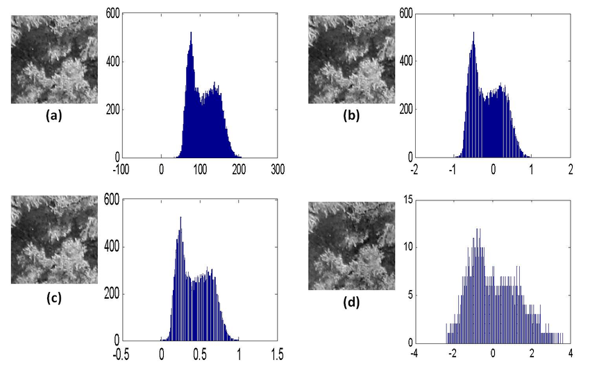
Normalization:
Normalizing images involves scaling the pixel values to a certain range, often between 0 and 1 or -1 and 1. This helps the model converge faster during training and stabilizes the optimization process. Here is the implementation part:
# Normalization
# Define a transformation that normalizes pixel values using mean and standard deviation
normalize_transform = transforms.Compose([
    transforms.Normalize(mean=[0.485, 0.456, 0.406], std=[0.229, 0.224, 0.225])
])
# Apply the normalization transformation to resized images
x_train_normalized = torch.stack([normalize_transform(img) for img in x_train_resized])
x_test_normalized = torch.stack([normalize_transform(img) for img in x_test_resized])
Here, a normalization transformation is defined using the specified mean and standard deviation values for each color channel. The transformation is constructed using transforms.Compose. The normalization is then applied to the resized images, resulting in x_train_normalized and x_test_normalized with pixel values scaled to a standard range.
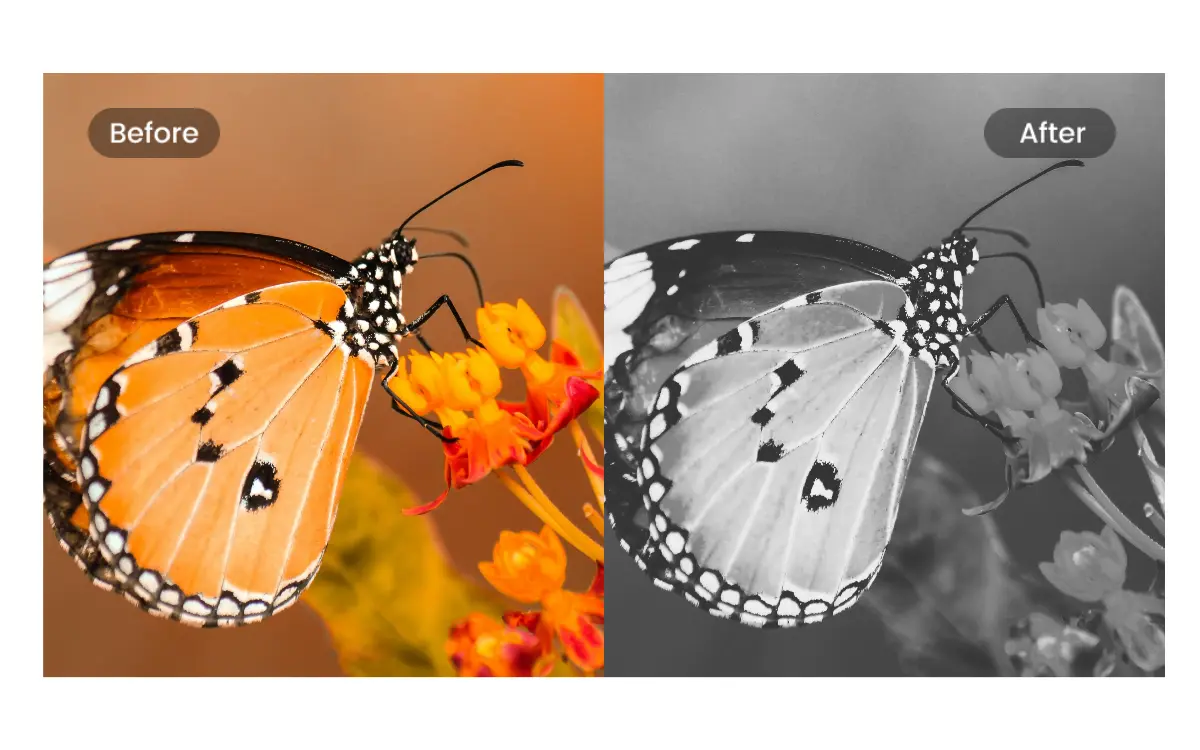
Grayscale Conversion:
Converting images to grayscale can simplify processing techniques, reduce memory requirements, and eliminate color-related variations that might not be relevant to the task. Here is the implementation part:
# Grayscale Conversion
# Convert RGB images to grayscale
x_train_grayscale = torch.stack([transforms.functional.rgb_to_grayscale(img) for img in x_train_normalized])
x_test_grayscale = torch.stack([transforms.functional.rgb_to_grayscale(img) for img in x_test_normalized])
This section performs an optional grayscale conversion of RGB images. The RGB images in x_train_normalized and x_test_normalized are converted into grayscale versions using the transforms—functional—rgb_to_grayscale function. Images produced in grayscale are saved under the names x_train_grayscale and x_test_grayscale.
Color Space Conversion: Changing the color space of an image, such as converting from RGB to HSV or LAB, can help extract specific information or improve performance in certain scenarios. For example, HSV separates color information from brightness, making it useful in tasks like object tracking. Here is the implementation part:
# Color Space Conversion
# For example, convert RGB images to HSV color space with slight color #jitter
hsv_transform = transforms.Compose([
    transforms.ToPILImage(),                        # Convert tensors to PIL images
    transforms.ColorJitter(hue=0.1, saturation=0.1, brightness=0.1),   # Apply color jitter
    transforms.ToTensor()                           # Convert modified images back to tensors
])
This coding part shows how to convert RGB photos to the HSV color space with a minor color jitter. This is an optional color space conversion. Using transforms, a transformation sequence is produced. Compose entails the transformation of tensors into PIL images, the application of color jitter with regulated fluctuations in hue, saturation, and brightness, and converting the altered images back to tensors. HSV_transform contains the entire transformation process.
Image preprocessing is a critical step in computer vision. In this tutorial, we describe the importance of image preprocessing, some image preprocessing tools, and image preprocessing techniques like resizing, grayscale conversion, normalization, and data augmentation that contribute to improved model performance. You can learn more about image preprocessing from here.