Machine Learning Project: Hotel Booking Prediction [Part 1]

Let’s Dive Into The Project

This is a hotel booking project where we will build a machine learning model to predict whether a booking made by a user is going to be canceled or not. In the dataset, there are several columns like arrival_date_time, stays_in_weekend, country, etc. With those huge chunks of data, we will predict our desired column ‘is_canceled’ result for each specific user. For getting the fantastic accurate model we will apply different supervised algorithms - KNN, LogisticRegression, Decision tree, and so on.

 For environment, setup follow this tutorial

Data Prepare for Analysis and Modelling

For this section, we are using hotel_bookings.csv as our dataset. We will perform several operations using this dataset.

 Download dataset from here

First, we have to clean our data because in the real-world aspect you won’t get clean data, the maximum time you will get raw or messy data. To build cool and fancy machine learning models you have to deal with them. In the Jupyter Notebook code section, we are importing some packages pandas, NumPy, matplotlib, and seaborn to extract, manipulate and visualize data for numerical computations, data visualization, and better visualization.

For doing operations, we have to read data by including a path into read_csv. This path tells us to read_csv where our dataset is located.

 

Pasting the path and adding file name at the end of the path by giving a ‘/’. Save the path into a variable and execute it.

If we want to see the first five rows of our data table we have to call the head() function.

To observe the total number of rows and columns in the table, we simply have to call shape.

Dealing with missing values

For checking the null value available in our dataset we have to use the isna() function that means is the null value available? And a sum function to do a summation of all the missing values in the dataset.

For dealing with these huge chunks of missing values we have to write a function named data_clean to fill the missing values using 0. This function will take df as input to update that missing value.

Now, we are going to watch the total column list by calling columns and have to consider three columns: adults, children, and babies to figure out the unique values of each and every column.

We will copy these columns and save them into a list for our next analysis. By running a loop over the entire list we can observe the unique values of each element.

This picture shows that we have noise in unique values, because adults, children, babies can’t have 0 in the list of the unique values at a time. We need to filter this.

Filtering missing values

We have used the set_option function to display entire columns. After that, we have filtered the adult, children, and babies columns.

Before Performing Spatial Analysis

When is_cancelled equals 0, that means it's a valid booking.

Passing this filter to the data frame to get the filter data frame.

We are accessing the country column and getting an idea about users.

Renaming column names for easy reading.

Spatial Analysis

We have used another library folium for visualizing. From that library, we are using plugins which are modules and imported HeatMap. By using a folium map we are retrieving our base map.

Used plotly for data visualization. Plotly is an advanced-level data visualization library that is extensively used for deployment-level visuals.

For performing spatial analysis two main functions are extensively used one is HeatMap and another is choropleth. It takes several parameters. First is coutry_wise_data, second locations cause we had to plot our countries to that map, third we added some color to our choropleth map on the basis of a number of guests, that means more the number of guests higher the density of that color will be, fourth hover parameter is added to reflect the field we want if you want country name/No of guests specify that, lastly added title.

How much do guests pay for a night analysis

Retrieving the first 5 rows of data.

We retrieved the is_canceled column for valid booking and saved it into a variable named data2.

Here we needed a price distribution of each room type. For that, we used the seaborn boxplot. By calling columns we achieved all the columns. From that info, we filled boxplot parameters. If you press shift+tab it will show all the parameters it takes, what is x, what is your y, and what is the hue parameter. Hue means on which column basis you have to split your boxplot.

Analyzing prices of hotels across the year

For this analysis, we considered resort hotels as well as city hotels. That means we need two data frames.

We passed our conditions into the data frame and checked if this was a valid booking or not.

To achieve ‘price per night varies over the year’, we had to check how exactly the price varies over the month because this is exactly similar to our problem statement. By considering the arrival_date_month column we have grouped our data frame.

The same operation has been done for city_hotel.

Merged both the data frame on the basis of arrival_date_month, cause both data frames has a common column name. For that, we had to call some in-built functions of pandas to make the merge function very useful.

                                                                                Fig 1

From Fig 1 we can see the month column isn’t in an arranged manner - means after April, May should come instead of August. So, we installed sorted-months-weekdays, sort-dataframeby-monthorweek packages. After that, we wrote a sort_data function that takes a data frame and column name as input parameters to solve this issue. Later, we called our sort_data function and passed the data frame and column name.

!pip install sorted-months-weekdays                 #Installing packages  
!pip install sorted-months-weekdays                 #Installing packages 
import sort_dataframeby_monthorweek as sd           #importing package and giving an alias
 
def sort_data(df,colname):                          #function taking inputs - dataframe and column name
    return sd.Sort_Dataframeby_Month(df,colname)    #returning sorted order of month
 
final=sort_data(final,'Month')                      #Calling the function and giving parameters
final                                               #printing the table

final.columns                   #Checking column names
px.line(final,x='Month',y=['Price_for_resort_hotel', 'Price_for_city_hotel'],title='Room price per night over the months')           
                                #plotting table using line

hix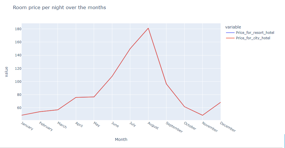

Analyzing Demand of Hotels

In this section, we tried to figure out which is the busiest month, which means in which month guests are highest. We considered our data frame for resort_hotel as well as city_hotel.

This is how our data frame looks like

data_resort.head()         #watching dataframe

Accessing the arrival_date_month feature for data_resort and converting it into a data frame. Source Code

rush_resort=data_resort['arrival_date_month'].value_counts().reset_index()     #accessing feature and converting into data frame
rush_resort.columns=['Month','No of guests']                                   #renaming column name
rush_resort                                                                    #printing the data frame

Accessing the arrival_date_month feature for data_city and converting it into a data frame.

rush_city=data_city['arrival_date_month'].value_counts().reset_index()     #accessing feature and converting into data frame
rush_city.columns=['Month','No of guests']                                 #renaming column name
rush_city                                                                  #printing the data frame

Here, we have merged data_resort with data_city on the basis of the month column and renamed the column name of the merged table. Then, sorted the month in a hierarchical manner.

final_rush=sort_data(final_rush,'Month')                                             #Sorting month column in hierarchical manner
final_rush.columns=['Month','No of guests in resort','No of guests of city hotel']   #Renaming new column name
final_rush=sort_data(final_rush,'Month')                                             #Sorting month column in hierarchical manner
final_rush

We figured out which is our busiest month. For that, we have used line plots to get the visualization on the basis of the month column.

final_rush.columns                             #Retrieving column name
px.line(final_rush,x='Month',y=['No of guests in resort', 'No of guests of city hotel'],title='Total number of guests per month')  
                                               #plotting to get perfect visualization trend

Select Important Features using Machine Learning

In this section, we have selected very important features using the correlation concept.

data.head()  #Showing data table

Finding correlation

data.corr()             #finding correlation

Finding correlation with respect to is_canceled. Here is_canceled is exactly our dependent feature, we can predict by using this feature that whether the booking is going to be canceled or not and easily figure out here how all these variables are going to impact on is_canceled feature. This is the exact meaning of correlation.

co_relation=data.corr()['is_canceled']       #finding correlation with respect to is_canceled
co_relation

Sorted correlation value in descending order and used abs to avoid all negative values.

co_relation.abs().sort_values()        #used abs to avoid negative values and sort_values to sort the value of correlation in 
                                       descending order

For, checking reservation status means Check-out, Canceled, and No-Show with respect to dependent variable ‘is_canceled’, we grouped by our data on the basis of ‘is_canceled’.

data.groupby('is_canceled')['reservation_status'].value_counts()        #Checking reservation_status on the basis of is_canceled

Fetched numerical features and categorical features separately for all the features. We excluded some variables for modeling purposes.

list_not=['days_in_waiting_list','arrival_date_year']                                          #excluding this feature
num_features=[col for col in data.columns if data[col].dtype!='O' and col not in list_not]     #fetching numerical colums num_features

Showing data columns

data.columns             #showing all columns

Excluding categorical features

cat_not=['arrival_date_year','assigned_room_type','booking_changes','reservation_status','country','days_in_waiting_list']     #excluding categorical columns                                                                                             
cat_features=[col for col in data.columns if data[col].dtype=='O' and col not in cat_not]        #list comprehension_cat_features     

How to extract Derived features from data

Extracted derived features from data

data_cat=data[cat_features]        #pushing cat_features to datafrmae
data_cat                                #executing 

Checking dtypes for next operation

data_cat.dtypes           #checking datatypes

import warnings
from warnings import filterwarnings                                     #importing filterwarnings from warnings package
filterwarnings('ignore')                                                #ingnoring warnings
data_cat['reservation_status_date']=pd.to_datetime(data_cat['reservation_status_date'])   #converting into datetime format and updating data_cat feature
data_cat.drop('reservation_status_date',axis=1,inplace=True)            #dropping reservation_status_date and updating by inplace true
data_cat['cancellation']=data['is_canceled']                            #inserting column
data_cat.head()

How to handle Categorical Data

For handling categorical data we are doing feature encoding on data. If we analyze the data table closely, we can see there are some string values in various columns. But machines can’t understand this, that’s why we convert this string into numerical form by applying feature encoding techniques. Mean encoding is one of the most popular encoding techniques we are using.

data_cat['market_segment'].unique()      #showing unique directory of market_segment

cols=data_cat.columns[0:8]   
cols                              #showing columns from 0 to 8 as we don't need cancellation column

data_cat['hotel']         #accessing hotels

for col in cols:
    print(data_cat.groupby([col])['cancellation'].mean())        #performing mean coding for each and every feature
    print('\n')

Converted all the features into a dictionary, because we had to map values. By converting it into a dictionary we achieved our data in a form of key: value pairs.

for col in cols:
    print(data_cat.groupby([col])['cancellation'].mean().to_dict())        #converting into dictionary
    print('\n')                                                            #added new line to make it more user friendly

for col in cols:
    dict=data_cat.groupby([col])['cancellation'].mean().to_dict()        #converted into dictionary
    data_cat[col]=data_cat[col].map(dict)                                #mapping the dictionary and updating data column

Here we can see that all our string values successfully converted into an integer values.

data_cat.head()          #for showing few rows

For working with real-world data, we need to apply an advanced approach. For this approach, we needed our entire data frame because that data frame includes all our categorical and numerical features.

dataframe=pd.concat([data_cat,data[num_features]],axis=1)     #concatenating in vertical fashion that's why axis=1
dataframe.head()                                              #dataframe showing

We dropped the ‘cancellation’ column as we already had the ‘is_canceled’ column.

dataframe.drop('cancellation',axis=1,inplace=True)             #dropping cancellation and updating dataframe by inplace true
dataframe.shape                                                #For showing shape of dataframe

This is the current shape of the data frame after dropping columns.

Click for the Hotel Booking Prediction project [Part 2]