Recent Articles
- Build Your First Machine Learning Project in Python(Step by Step Tutorial)
- Build and Deploy a Restaurant Chatbot with Rasa and Python
- A Quick Guide to Deploy your Machine Learning Models using Django and Rest API
Learn Time Series Analysis in Python- A Step by Step Guide using the ARIMA Model
Written by - Aionlinecourse8684 times views
Recommended Projects
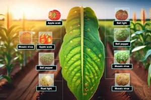
Crop Disease Detection Using YOLOv8
In this project, we are utilizing AI for a noble objective, which is crop disease detection. Well, you're here if...
Computer Vision

Topic modeling using K-means clustering to group customer reviews
Have you ever thought about the ways one can analyze a review to extract all the misleading or useful information?...
Natural Language Processing

Optimizing Chunk Sizes for Efficient and Accurate Document Retrieval Using HyDE Evaluation
This project demonstrates the integration of generative AI techniques with efficient document retrieval by leveraging GPT-4 and vector indexing. It...
Natural Language ProcessingGenerative AI

Skin Cancer Detection Using Deep Learning
Think about it if diagnosing skin cancer could be done by uploading a picture of the skin. In this project,...
Deep Learning

Automatic Eye Cataract Detection Using YOLOv8
Cataracts are a leading cause of vision impairment worldwide, affecting millions of people every year. Early detection and timely intervention...
Computer Vision

Medical Image Segmentation With UNET
Have you ever thought about how doctors are so precise in diagnosing any conditions based on medical images? Quite simply,...
Computer Vision

Real-Time License Plate Detection Using YOLOv8 and OCR Model
Ever wondered how those cameras catch license plates so quickly? Well, this project does just that! Using YOLOv8 for real-time...
Computer Vision