Generative Adversarial Networks (GANs) | Generative AI

Introduction

An innovative method for generative modelling in artificial intelligence, generative adversarial networks. In an effort to transform artificial intelligence and machine learning, this blog will examine the complexities, elements, functions, applications, benefits, and drawbacks of GANs.

Importance of Generative Adversarial Networks (GANs)

Artificial intelligence's generative adversarial networks (GANs) are transforming generative modelling and content generation. They solve data privacy issues, create synthetic data, and improve model robustness. GANs are influencing and developing artificial intelligence in a variety of fields, including entertainment, science, and the democracy of AI.

Understanding Generative Adversarial Networks (GANs)

The Generator and Discriminator neural networks interact dynamically to form the basis of GANs. The generator's job is to produce artificial intelligence generated text or graphics that closely mimic genuine data. As a critic, on the other hand, the discriminator distinguishes between data produced by the generator and actual data from a training dataset.

A competitive game can be used to describe the training process of GANs. Concurrently, the discriminator works to improve its capacity to discern between authentic and fraudulent data, while the generator aims to generate samples that are ever more realistic. Both networks' performance increases as a result of this adversarial training, which creates a loop of progress.

Components and Architecture of GANs

The generator and discriminator models, which combine convolutional layers to assess the authenticity of input samples and convert random noise into meaningful data samples, make up a generalized autonomous network. Different GAN designs are designed for different datasets and applications, including Vanilla GAN, Conditional GAN, DCGAN, LAPGAN, and SRGAN.

Applications of GANs

The versatility of GANs transcends traditional boundaries, offering a plethora of applications across diverse domains:

• Image Synthesis and Generation: High-resolution pictures, avatars, and artwork may be produced using GANs' ability to produce realistic visuals that closely resemble real-world data distributions.
• Image-to-Image Translation: GANs make it easier to convert pictures between domains while maintaining important aspects, enabling changes like night-to-day conversion or style transfer.
• Text-to-Image Synthesis: Generating realistic material based on textual input is made possible by GANs' ability to create visual representations from textual descriptions.
• Data Augmentation: GANs improve the generalizability and robustness of machine learning models by producing synthetic data samples, especially in situations when there is a shortage of labelled data.
• Data Generation for Training: GANs provide higher picture quality in applications like medical imaging, satellite imaging, and video enhancement by increasing the resolution and quality of low-resolution images.

Architecture of GANs

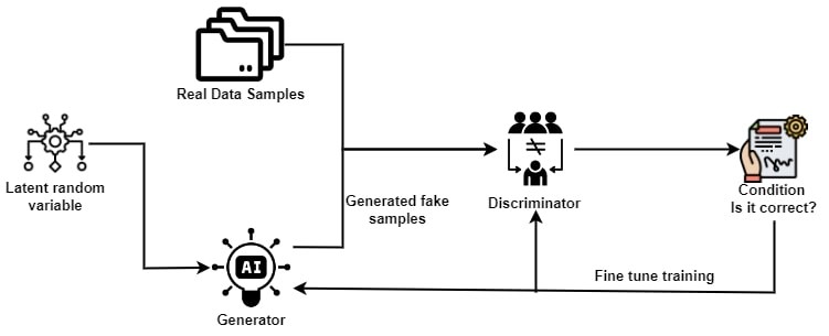
The generator and the discriminator are the two main components that make up a generative adversarial network.

Generator Model

A GAN's generator is essential for producing realistic data since it converts random noise into intricate samples like text or graphics. Through training, it acquires the ability to replicate the fundamental distribution of authentic data, modifying its parameters to produce superior examples that trick the discriminator.

Generator Loss

The goal of a GAN's generator is to provide plausible samples that trick the discriminator. By increasing the log probability, it minimises its loss function, JG guaranteeing that the discriminator will most likely categorise produced samples as real.

JG​=−m1​Σi=1m​logD(G(zi​))

Where,

• The generator's ability to trick the discriminator is measured by JG.
• For generated samples, the log likelihood of the discriminator being correct is represented by logD(G(zi​)).
• In order to reduce this loss, the generator produces samples that are classified as real (logD(G(zi​)​)​), near 1, by the discriminator.

Discriminator Model

A discriminator model is used by Generative Adversarial Networks (GANs) as a binary classifier to distinguish between generated and real input. As it gains experience, the discriminator becomes more adept at differentiating between real data and artificial samples. Its architecture usually uses convolutional layers for image data. In order to produce realistic synthetic data, the adversarial training procedure tries to maximise the discriminator's capacity to correctly classify generated samples as authentic and fraudulent.

Discriminator Loss

The discriminator reduces the likelihood of correctly classifying both produced and real samples, incentivizing accurate classification of generated samples using the following equation:

JD​=−m1​Σi=1m​logD(xi​)-m1​Σi=1m​log(1-D(G(zi​))

The discriminator's capacity to distinguish between manufactured and real samples is evaluated by JD.

• A discriminator's log probability of correctly classifying actual data is given by ​logD(xi​).
• log⁡(1−D(G(zi​))) represents the log likelihood that the discriminator will properly classify produced data as false.
• With precise identification of fake and genuine samples, the discriminator seeks to minimise this loss.

MinMax Loss

The minimax loss formula in a generative adversarial network (GAN) is given by:

minG​maxD​(G,D)=[Ex∼pdata​​[logD(x)]+Ez∼pz​(z)​[log(1-D(g(z)))]

Where,

• The discriminator network is D, while the generator network is G.
• x represents actual data samples that were taken from the genuine data distribution pdata​(x).
• Z represents random noise collected from a previous distribution pz​(z).
• The discriminator's probability of accurately classifying actual data as real is represented by D(x).
• The probability that the discriminator will recognize produced data from the generator as legitimate is D(G(z)).

Workflow:

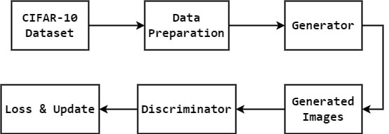
Here's a simplified overview:

CIFAR-10 Dataset:

• The CIFAR-10 dataset is the source of real images.

Data Preparation:

• Data from CIFAR-10 is prepared for training, which includes normalization and transformation.

Generator:

• Takes random noise as input and generates fake images.

Generated Images:

• These are the images generated by the generator.

Discriminator:

• Receives both real images (from the dataset) and fake images (from the generator).
• It classifies these images as real or fake.

Loss & Update:

• Based on the discriminator's classification, the generator and discriminator update their weights to improve performance.

This basic figure shows how it works: actual images from CIFAR-10 are used to train the discriminator, which then feeds back information to the generator to produce more lifelike false images. Up till the generator and discriminator both get better, the process is repeated.

Implementation of Generative Adversarial Network (GAN)

Step1 : Importing the required libraries

This code configures the device, checks for GPU availability, and sets up PyTorch for image tasks. It imports 'matplotlib' and 'numpy' for visualization, 'torchvision' for datasets, and PyTorch modules for neural networks and optimization. Effective deep learning requires this, particularly for image-based tasks.

import torch
import torch.nn as nn
import torch.optim as optim
import torchvision
from torchvision import datasets, transforms
import matplotlib.pyplot as plt
import numpy as np
# Set device
device = torch.device('cuda' if torch.cuda.is_available() else 'cpu')

Step 2: Defining a Transform

Using a mean and standard deviation of 0.5, this method converts images to PyTorch tensors in order to prepare them for deep learning models.

transform = transforms.Compose([
transforms.ToTensor(),
transforms.Normalize((0.5, 0.5, 0.5), (0.5, 0.5, 0.5))
])

Step 3: Loading the Dataset

Using CIFAR-10 and the specified transformation, this code generates a training dataset (‘train_dataset’), then loads it into a ‘DataLoader’ (‘dataloader’) for batching with a size of 32 and shuffling.

train_dataset = datasets.CIFAR10(root='./data',\
              train=True, download=True, transform=transform)
dataloader = torch.utils.data.DataLoader(train_dataset, \
                                batch_size=32, shuffle=True)

Step 4: Defining parameters to be used in later processes

These hyperparameters, ‘latent_dim’, ‘lr’, ‘num_epochs’, ‘beta1’, and ‘beta2’, are essential for GAN training, influencing image quality.

latent_dim = 100
lr = 0.0002
beta1 = 0.5
beta2 = 0.999
num_epochs = 10

Step 5: Defining a Utility Class to Build the Generator

The ‘Generator’ class in a GAN transforms a latent vector ‘z’ into realistic images using fully connected and convolutional layers with ReLU activations, batch normalization, and a ‘Tanh’ output. It converts noise to images during GAN training.

# Define the generator
class Generator(nn.Module):
def __init__(self, latent_dim):
super(Generator, self).__init__()
self.model = nn.Sequential(
nn.Linear(latent_dim, 128 * 8 * 8),
nn.ReLU(),
nn.Unflatten(1, (128, 8, 8)),
nn.Upsample(scale_factor=2),
nn.Conv2d(128, 128, kernel_size=3, padding=1),
nn.BatchNorm2d(128, momentum=0.78),
nn.ReLU(),
nn.Upsample(scale_factor=2),
nn.Conv2d(128, 64, kernel_size=3, padding=1),
nn.BatchNorm2d(64, momentum=0.78),
nn.ReLU(),
nn.Conv2d(64, 3, kernel_size=3, padding=1),
nn.Tanh()
)
def forward(self, z):
img = self.model(z)
return img

Step 6: Defining a Utility Class to Build the Discriminator

In a GAN, the 'Discriminator' employs convolutional layers, leaky ReLU activations, dropout, and batch normalization to process input images. A fully linked layer and 'Sigmoid' activation for real/fake probability mark the end of it. During GAN training, this model picks up classification skills for images.

# Define the discriminator
class Discriminator(nn.Module):
def __init__(self):
super(Discriminator, self).__init__()
self.model = nn.Sequential(
nn.Conv2d(3, 32, kernel_size=3, stride=2, padding=1),
nn.LeakyReLU(0.2),
nn.Dropout(0.25),
nn.Conv2d(32, 64, kernel_size=3, stride=2, padding=1),
nn.ZeroPad2d((0, 1, 0, 1)),
nn.BatchNorm2d(64, momentum=0.82),
nn.LeakyReLU(0.25),
nn.Dropout(0.25),
nn.Conv2d(64, 128, kernel_size=3, stride=2, padding=1),
nn.BatchNorm2d(128, momentum=0.82),
nn.LeakyReLU(0.2),
nn.Dropout(0.25),
nn.Conv2d(128, 256, kernel_size=3, stride=1, padding=1),
nn.BatchNorm2d(256, momentum=0.8),
nn.LeakyReLU(0.25),
nn.Dropout(0.25),
nn.Flatten(),
nn.Linear(256 * 5 * 5, 1),
nn.Sigmoid()
)
def forward(self, img):
validity = self.model(img)
return validity

Step 7: Building the GAN

This code sets up a GAN with a 'Generator' and 'Discriminator'. The 'Generator' takes a 'latent_dim' input and is moved to 'device'. The GAN uses BCE loss ('adversarial_loss') and Adam optimizers ('optimizer_G', 'optimizer_D') with defined parameters ('lr', 'beta1', 'beta2'). These components are essential for training the GAN to generate realistic images and improve discrimination between real and generated ones.

generator = Generator(latent_dim).to(device)
discriminator = Discriminator().to(device)

adversarial_loss = nn.BCELoss()

optimizer_G = optim.Adam(generator.parameters()\
, lr=lr, betas=(beta1, beta2))
optimizer_D = optim.Adam(discriminator.parameters()\
, lr=lr, betas=(beta1, beta2))

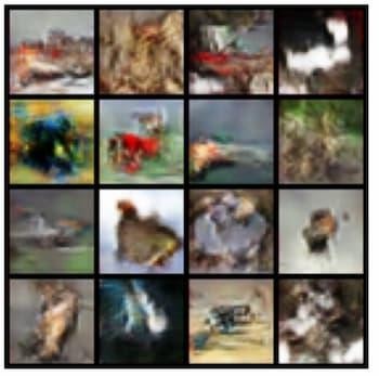
Step 8: Training the GAN

This code trains a GAN with a Discriminator and Generator. The Discriminator learns to distinguish real from generated images using BCE loss (adversarial_loss). The Generator creates images to fool the Discriminator, optimizing with the same loss. Both models' weights are updated for improved image generation and discrimination. Losses are printed every 100 batches, and every 10 epochs, 16 generated images are displayed for evaluation.

for epoch in range(num_epochs):
for i, batch in enumerate(dataloader):

real_images = batch[0].to(device)

valid = torch.ones(real_images.size(0), 1, device=device)
fake = torch.zeros(real_images.size(0), 1, device=device)

real_images = real_images.to(device)
# ---------------------
# Train Discriminator
# ---------------------
optimizer_D.zero_grad()

z = torch.randn(real_images.size(0), latent_dim, device=device)

fake_images = generator(z)

real_loss = adversarial_loss(discriminator\
(real_images), valid)
fake_loss = adversarial_loss(discriminator\
(fake_images.detach()), fake)
d_loss = (real_loss + fake_loss) / 2
# Backward pass and optimize
d_loss.backward()
optimizer_D.step()

# -----------------
# Train Generator
# -----------------
optimizer_G.zero_grad()

gen_images = generator(z)

g_loss = adversarial_loss(discriminator(gen_images), valid)

g_loss.backward()
optimizer_G.step()

# ---------------------
# Progress Monitoring
# ---------------------
if (i + 1) % 100 == 0:
print(
f"Epoch [{epoch+1}/{num_epochs}]\
Batch {i+1}/{len(dataloader)} "
f"Discriminator Loss: {d_loss.item():.4f} "
f"Generator Loss: {g_loss.item():.4f}"
)

if (epoch + 1) % 10 == 0:
with torch.no_grad():
z = torch.randn(16, latent_dim, device=device)
generated = generator(z).detach().cpu()
grid = torchvision.utils.make_grid(generated,\
nrow=4, normalize=True)
plt.imshow(np.transpose(grid, (1, 2, 0)))
plt.axis("off")
plt.show()

output:

Epoch [10/10]                   Batch 1300/1563 Discriminator Loss: 0.4473
Generator Loss: 0.9555
Epoch [10/10]                        Batch 1400/1563 Discriminator Loss: 0.6643
Generator Loss: 1.0215
Epoch [10/10]                        Batch 1500/1563 Discriminator Loss: 0.4720
Generator Loss: 2.5027

Advantages and Limitations of GANs

Advantages:

• GANs may produce synthetic data that mimics well-known distributions, which helps in anomaly identification and data augmentation.
• Across a range of jobs, they generate excellent, lifelike results.
• Because GANs are trained on unlabeled data, they are appropriate for applications involving unsupervised learning.
• They are versatile in their applications, encompassing text production and image synthesis.

Limitations:

• GANs pose a danger of instability and mode collapse, making training them challenging.
• They require a large amount of processing power, particularly for high-resolution photos.
• GANs may reflect biases in the data and overfit training sets.
• It is difficult to guarantee justice and accountability because of their opaqueness and lack of interpretability.

Conclusion

Absolutely, generative adversarial networks have transformed artificial intelligence by enabling hitherto unheard-of potential in generative modeling and the creation of creative content. GANs are pushing the envelope of machine learning capabilities by creating realistic image synthesizers and turning text into pictures. We may anticipate further developments that will influence the direction of AI-driven creativity and innovation as scholars and practitioners dive deeper into the nuances of GANs.